O&M

A Primer on Optimizing Fleet Operations

The power industry needs a straightforward definition of "fleet optimization" and a game plan to achieve the promised economic gains of optimizing. This need has become more urgent because integrating nondispatchable renewable resources requires more complex optimization strategies. The bottom-up approach presented here applies well-understood optimization principles and techniques that will help power producers minimize their fleetwide cost of production, independent of the technologies used to generate electricity.

If your utility, company, municipality, cooperative, or government agency owns or operates one or more power generating units, then it has a fleet operating in a market. A vertically integrated utility is in essence a market unto itself; its interties with other utility grids, regional transmission organizations (RTOs) and independent system operators (ISOs) can be modeled as virtual units in the utility’s fleet. Each of the competitive wholesale markets run by RTOs and ISOs in the U.S. is also defined as a market with a fleet of generating units competing to supply the demanded energy. Therefore, a company that owns units in PJM and in ISO New England has two fleets. In addition, a unit with more than one owner may be part of many fleets, one for each owner, but each unit typically competes in only one market. For the purposes of this discussion, please assume that our demonstration fleet operates in a single market, such as PJM or MISO.

Focus on Lowest Cost

Optimization is the process of minimizing or maximizing some quantity, given a set of relationships between variables and a set of constraints that must be satisfied. Together, the set of relationships and the set of constraints is called an optimization problem. This is a somewhat theoretical definition, but it is a very powerful tool. It means that if you are not seeking to minimize or maximize some quantity, then you are not optimizing. This may seem to be a silly distinction, but it turns out to be important in every optimization problem because of the trade-offs that are inherent in the set of relationships between variables.

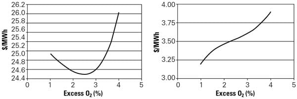
As an example, consider that you can reduce the amount of NO_x produced in a boiler’s furnace by reducing the amount of excess air used for combustion (Figure 1). As excess air is reduced, a coal-fired boiler produces more unburned carbon in the ash. More unburned carbon in the ash means the heat rate has increased or the combustion efficiency has decreased. Therefore, we can tune the combustion to minimize NO_x or we can tune the combustion to minimize unburned carbon, but we can’t minimize both at the same time. Optimization tools provide us with a methodology to balance competing plant operating practices, such as minimizing NO_x and unburned carbon, to achieve the overall lowest cost to a particular boiler and, eventually, to the entire fleet of plants.

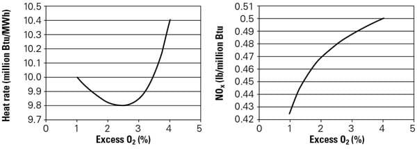
1. Characterize the test data. The first step is to characterize the important data used to define unit performance. In this example, the amount of excess O₂ in the boiler furnace determines the plant heat rate (left) and NO_x production (right). Note that it’s impossible to minimize the plant heat rate and NO_x emissions at the same furnace excess O₂. Source: Emerson Process Management

There are costs associated with creating NO_x in a boiler and unburned carbon in the ash. Those costs may come from purchasing or maintaining NO_x emission allowances, buying ammonia for selective catalytic reduction (SCR), or limiting a unit’s power output to stay under a NO_x cap or rate limit (Figure 2). Quantifying the universe of costs related to NO_x production, for example, may be easy or extremely difficult, but there is no question that system operating costs increase as more NO_x is produced (Figure 3). Similarly, there is a cost associated with unburned carbon. The more carbon that is thrown out with the ash, the more it costs in fuel for each megawatt-hour produced.

2. Find the incremental cost. The same variables used in Figure 1 can be used to determine the fuel cost (left) and the incremental additional cost of NO_x, including the cost of allowances, as a function of excess O₂ in the boiler furnace. Source: Emerson Process Management

3. Find the optimum settings. With the data from Figure 2, an equation for the total cost of production as a function of excess O₂ is possible. The minimum production cost defines the optimum setting as 2.26% O₂ in the boiler furnace, resulting in a total production cost of $28.01/MWh. Source: Emerson Process Management

The process of optimizing these competing requirements to the benefit of the entire fleet requires minimizing the total costs associated with NO_x and unburned carbon while satisfying all the NO_x emissions limits applicable to the unit. The dollar is the conversion factor that allows us to find the sweet spot in this trade-off.

A very complicated set of mathematical relationships encompassing many variables (such as NO_x production or unburned carbon in the ash) ultimately determines all the costs associated with making electricity at a plant or in a fleet. There is also an extensive set of process constraints (such as annual NO_x production limits) that must be satisfied in any optimization problem. In the short term, fleet optimization is a matter of formulating and solving the optimization problem to minimize short-term or variable costs while satisfying all the constraints. In the midterm, there may be other fixed costs associated with short-term optimization. Midterm optimization is the process of minimizing all costs, accounting for these fixed costs in combination with the variable costs.

Use the Existing EMS System

In tackling the fleet optimization problem, begin with a bottom-up approach that leverages one optimization tool that every fleet already has at its disposal. The utility’s or ISO’s energy management system (EMS) now dispatches all the power generation resources, regardless of whether they are used in a nonmerchant utility fleet or in a competitive wholesale market.

The EMS utilizes a rigorous solution method that guarantees least-cost dispatch of the fleet, given the relationship between cost and load for each unit and a set of constraints describing the minimum load, maximum load, typical ramp rate, start-up time, and a host of other constraints applicable to each unit. In sum, the fleet achieves the minimum cost of production when each unit has optimized to its minimum cost and the fleet as a whole can change its output as required by the changing demand of customers while maintaining a minimized cost dispatch solution. To maintain a combination of operating units (or purchased power) that produces the lowest possible energy cost while following a daily load demand curve is a valuable capability.

To illustrate, consider a fleet supplying electricity into a market during a period of rising demand. If a low-cost-of-energy unit cannot keep up with the increasing demand, then a higher-cost-of-energy unit must generate more energy than the least-cost ideal arrangement for the fleet, in order to balance energy supply with demand at every instant in time. Thus, the total cost of energy for the fleet is higher than it would have been if the low-cost unit could keep up with the rate of change of demand.

One important observation from this discussion: The fleet can be optimized only when each unit in the fleet is locally optimized throughout its operating range.

Short-Term Unit Optimization

We begin optimizing an individual unit based on short-term operating goals. This approach requires definition of all of the relationships between variables that determine plant variable operating costs, within the required operating constraints. For most units, these variable costs of producing electricity include commodities that are either purchased or otherwise procured. Examples include:

Fuel
NO_x allowances
SCR or selective noncatalytic reduction r agent (ammonia or another reagent)
SO₂ allowances
Flue gas desulfurization (FGD) reagent (limestone, lime, or other chemical consumables)

Some units have variable costs associated with the purchase of water used for cooling water and FGD slurry water. The portion of that water that represents a variable cost is typically what is evaporated or otherwise consumed as a function of plant energy (MWh) production. Some locations also inject reagents such as activated carbon to reduce mercury emissions, so those costs should also be included, if applicable. Future carbon cap-and-trade regulations may also create a significant variable cost in the cost to produce electricity.

Calculations are further complicated for units located in states that do not have tradable allowances but that do place limits on emissions. The variable or incremental cost to replace power lost when a unit runs up against a NO_x limit (whether hourly or daily) is the virtual value of the NO_x allowances used.

For example, consider Unit #1, which generated 600 MWh over the past hour but would have generated 800 MWh had it not been for a NO_x limit. Suppose that Unit #2, with an additional incremental cost of $5.25/MWh, generated the 200-MWh difference. Also, Unit #1 would have made an incremental three pounds of NO_x per MWh for a total increment of 600 lb of NO_x during the hour. Thus, the ability to emit NO_x from Unit #1 is valued as:

$5.25/MWh * 200 MWh/600 lb NO_x = $1.75 per pound of NO_x, or $3,500 per ton of NO_x

In the optimization of Unit #1, a cost of $3,500 per ton of NO_x would be used to find the "sweet spot" in the combustion optimization trade-off.

Continuing with Unit #1, there are many adjustments that an operator or a control system can make to produce the lowest possible cost of electricity, such as damper positions, fan speeds, and burner tilt, to name a few. In the language of optimization science, these are called "manipulated variables." Changes in the manipulated variables change the plant "dependent variables," such as flue gas oxygen content, steam temperatures, heat transfer surface cleanliness, and the like. Changes in dependent variables usually result in changes to other dependent variables and so on, down a long chain of relationships that ultimately produce a change to the cost of electricity production.

The total cost of electricity production is the ultimate dependent variable, and our objective is its minimization. Other "disturbance variables" such as ambient temperature and humidity, condenser cooling water inlet temperature, and water content of the fuel also produce effects on the dependent variables, and those effects must be characterized in order to achieve our optimization objective. The combination of all the mathematical characterizations of each of these variables is called the "objective function." The solution of the objective function yields settings for all of the manipulated variables so that the cost to produce a MWh is minimized (Figure 4).

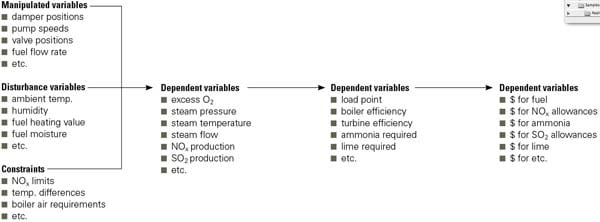
4. The objective is to minimize cost. The mathematical approach to fleet optimization is to define an objective function that is cost-minimized. In addition, the program must characterize each dependent variable as a function of manipulated, disturbance, and other dependent variables. The constraints must also be defined as part of the analysis. Source: Emerson Process Management

The Importance of Data Handling

Any plant performance engineer who tried to tackle unit optimization prior to about 1992 will testify that the multitude of functional relationships between the variables and the continuous data stream required was overwhelming. Fortunately, we now have the computing power necessary, at an affordable cost, to characterize the responses of the dependent variables to changes in the manipulated and disturbance variables, to develop the objective function as a set of mathematical expressions, and to perform the mathematics required to solve these complex equations to determine settings for the manipulated variables every few seconds.

In order to minimize the total variable cost, detailed information about the cost of the commodities listed above must be supplied to unit optimization programs. The programs that collect the data and develop the characterizations are called "neural networks" or "artificial intelligence" or some variation on that theme. A neural network is a program that gathers data, characterizes responses to manipulations and disturbances, and then uses those characterizations to produce the ideal desired result. In effect, the computer program "learns" how to respond to complex situations based on historic data. Some newer programs add the capability to recognize when something about the process has changed. When a process variable changes, the program immediately develops new characterizations of the data that are used to "immunize" the optimization problem against that change going forward.

Short-Term Fleet Optimization

Even using state-of-the-art optimization computer programs, characterizing a unit and producing a bulletproof optimizer is not a trivial exercise. However, it is possible — and even reasonably economical — today, since robust computer tools are now available. Having characterized the settings (the manipulated variables) required to minimize real-time total cost of production for each unit, the characterization of cost as a function of unit load can be supplied to the fleet EMS (Figure 5).

5. Grade on the curve. Once commodity prices and actual equipment performance are included in the analysis, each unit’s incremental cost curve defines the true cost of production by unit. That data can then be used by the fleet EMS to dispatch the units. Source: Emerson Process Management

Traditionally, the cost of fuel across the load range has been the only commodity represented in this characterization. With the advent of emissions cap-and-trade systems and the cost of emissions reduction reagents used in SCRs and scrubbers, this one-dimensional approach is no longer adequate. A properly configured unit optimization system should output, or at least provide access to, the necessary information to produce near-real-time characterizations of cost as a function of load that includes all variable costs. Once the settings for the manipulated variables are determined, the EMS then takes care of dispatching each unit at the load necessary to minimize the total real-time cost of the fleet.

The first challenge in fleet optimization (as distinct from unit optimization) is to update the EMS with fresh characterizations of the units, whenever it’s appropriate. This means that each unit optimizer must be able to recognize when something about its objective function has changed enough to cause a change in the unit characterization used by the EMS. Almost any change in the performance of any power plant equipment will cause the objective function to change. Examples include a stuck overfire air damper, a change in boiler feed pump efficiency due to wear, and a leak in a start-up drain valve.

Any change in the cost of any of the variable cost commodities also causes the objective function to change. Because these quantities change frequently, the EMS must have near-real-time updates of each unit’s cost characteristics. Unit optimizers or control systems that automatically feed near-real-time cost characteristics to an EMS are uncommon in the industry, but it’s important to realize that fleet optimization is performed by the EMS, so real-time, accurate unit incremental cost curves must be provided. A unit that is dispatched by an EMS using an inaccurate incremental cost curve loses money in the market and increases the fleet’s aggregate cost.

Midterm Fleet Optimization

Having successfully achieved short-term fleet optimization, we turn our attention to optimization in the midterm. The goal here is to understand how changes in operating procedures might change a unit’s objective function for the better, or might change some operating constraint in a way that produces a lower-cost result from the EMS. The typical trade-off is a rising cost of unit maintenance. A good example is a potentially costly side effect of combustion optimization.

Recalling our earlier example, reducing excess O₂ can reduce the amount of NO_x produced, and we optimized the unit by pushing that benefit until the cost of unburned carbon balances the benefit of reduced NO_x. A midterm consequence of this short-term optimization can be an increase in tube wastage caused by alternating oxidizing and reducing atmospheres in the furnace (Figure 6). Some units have experienced a significant increase in tube leaks that increase tube repair maintenance costs and reduce the operating reliability of the entire unit. Also, when a unit is forced offline to repair a tube leak, it misses the opportunity to generate revenue in the market, thereby increasing the fleet’s "reliability costs." These costs are incremental to the cost of operations and maintenance incurred when running with higher O₂.

6. Include long-tem effects. Short-term optimization of variable costs often ignores the longer-term effects, such as boiler water wall tube wastage that takes place over years. Operating at low boiler furnace O₂ levels accelerates tube wastage (left) and the resultant cost of replacement on an incremental cost basis (right). For this analysis, the tube replacement cost was estimated as $12 million on a 600-MW unit operating at 75% capacity factor. Source: Emerson Process Management

Midterm fleet optimization then can be an exercise in the minimization of the costs resulting from short-term optimization added to any incremental maintenance and reliability costs resulting from the short-term optimization. Of course, the main difficulty with midterm optimization is that it takes a while to measure the effects of a given decision.

Continuing with our tube leak example, suppose we start with a unit whose water walls are expected to remain serviceable for 30 years of baseload operation, at 3% minimum economizer O₂. Suppose further that our efforts at short-term optimization indicate that operating at 2.3% O₂ would result in NO_x allowance and fuel savings amounting to $850,000 per year. Assume that we know that an outage to replace all of the degraded tubes would cost $12,000,000 in material, labor, replacement power, and all the other associated costs. A hypothetical wastage rate curve allows us to estimate the cost per MWh of the tube wastage as a function of excess O₂ (Figure 7).

7. Combine long- and short-term costs. The optimum boiler furnace O₂ setpoint can now be determined by summing the short-term unit optimization data that minimized variable O&M cost (Figure 3) with the midterm fleet optimization that consider fixed O&M costs (Figure 6). Doing so results in an overall production cost optimization strategy that encompasses furnace O₂, NO_x, and tube wastage. In this example, the optimum furnace O₂ is 2.48% at a cost of $28.10/MWh. The estimated interval between tube replacements is 18.43 years. This analysis shows that the unit will save $494,000 per year against the boiler manufacturer’s suggested 3% furnace O₂ setpoint by minimizing the total costs of fuel, NO_x allowances, and tube replacements. Source: Emerson Process Management

With this relationship added to the short-term optimization problem, we will now control O₂ at the point that minimizes the total of the short-term costs of fuel and NO_x allowances plus the midterm costs of tube replacement events. A "conservative" approach in terms of protecting the boiler would be to estimate a high rate of tube wastage, driving the optimization solution away from 2% and closer to 3% O₂, at the risk of leaving NO_x allowance or fuel money on the table.

A more aggressive approach would be to estimate a less "conservative" wastage effect, driving the solution toward the short-term optimum. Then, taking a short outage every year to perform ultrasonic testing and characterize the wastage rate would provide the information needed to adjust the wastage relationship, leading to a better characterization of tube repair costs and a lower total cost optimum. This sort of process is the essence of a continuous improvement program, approached from a perspective that combines business and engineering sciences. It is applicable to any number of operations versus maintenance trade-off situations, including reduction of minimum load, unit load ramp rate, and cycling operations.

With a clear understanding of midterm cost characteristics, the variable cost curves of each unit in a fleet can then be adjusted to reflect both short-term and midterm costs. The update ensures the appropriate unit dispatch order to minimize fleet cost of production over the midterm.

This approach also addresses one of the most difficult issues between plant management and dispatch or trading management. Commonly, either the plant gives the dispatcher whatever he wants and then blames "erratic dispatch" for a high forced outage rate, or the plant constrains dispatch in an effort to minimize damage to the equipment but leaves big money on the table in terms of the ability to minimize fleetwide aggregate cost of production. Midterm fleet optimization offers the mechanism through which the fleetwide lowest total cost set of constraints and operating settings are used by the unit optimizers and the EMS.

Some companies have rejected short-term optimization, fearing that the resulting midterm costs might become too high. To reject short-term optimization on that basis is to reject the notion that there is room to improve the operating economics of the fleet. Midterm optimization provides the means to replace this fear-based decision-making with knowledge-based or at least reason-based decision-making.

—Tom Snowden ([email protected]) is a performance consultant with the Power & Water Solutions division of Emerson Process Management.