Desalination, Italian style
Reverse osmosis (RO) technology has been available for all aspects of water treatment for the past 40 years. The use of RO desalination systems grew rapidly following their commercialization in the 1960s. The first thin-film composite membranes were introduced in the mid-1970s, and the first seawater systems were built later in the decade. Early seawater systems consisted of two passes or a partial second pass because their membranes, even operating at 99% salt rejection, could not produce potable water in one pass.
Since then, design refinements have increased membrane flux and salt rejection, allowing production of low-salinity water in one pass. Concurrently, improvements in RO membrane construction—including spiral-wound elements—enabled operation at higher pressures (up to 1,200 psi), raising recovery rates from high-salinity water. By the late 1990s, it became clear that a high-flux seawater membrane able to convert low-salinity seawater to power plant process water and boiler makeup would be widely adopted in many markets for its capital and operating cost advantages.
Italy was one such market. The wholesale switch from coal to oil by power plants there in the 1990s created a need to have de-SOx plants available on-site for flue gas scrubbing. The addition of the de-SOx trains, in turn, changed the plants’ requirements for water volume and quality.
One example is the six-unit, 1,280-MW San Filippo del Mela plant in Sicily. Since its commissioning between 1971 and 1976, it had used demineralization and mixed-bed ion exchange systems to convert well water to boiler makeup. But the new de-SOx plant installed on-site required more process water than the well or those systems could provide. Complicating the problem, the quality of water needed by the de-SOx plant was much lower than that required for boiler makeup. Whereas the former needed water with a conductivity of no more than 1,000 microsiemens (micromhos) per centimeter (µS/cm), boiler makeup had to be less than 20 µS/cm.
RO beats heat
Realizing that switching to desalinated seawater was the only option, Edipower SpA (the San Filippo plant’s operator at the time) decided in favor of treating it using a membrane system rather than a thermal desalination process. The seawater RO system chosen—a Fluid Systems TFC 2822F-370 from Koch Membrane Systems Inc. (Wilmington, Mass.)—uses a partial second pass, as opposed to evaporators, due to the need for water of two different qualities. The 1.38 million-gallon-per-day system, which was commissioned in 2000, also is notable for its high-flow, 8-inch-high seawater elements, among the first to see commercial service anywhere.
The seawater that serves as the system’s "feedstock" is drawn from 820 feet out in the Mediterranean at a depth of 50 to 65 feet. The seawater, at a temperature of 50F to 80F, typically has about 42,000 mg/l of total dissolved solids and a conductivity of 57,000 µS/cm. First, it is pretreated, by dosing with sodium hypochlorite for disinfection and (optionally) with a polyelectrolyte to improve coagulation.
Next come three stages of filtration. In the first, the pretreated seawater is continuously backwashed through up-flow gravity sand filters. The filtered water is collected in a tank and then pumped through second-stage multimedia pressure sand filters, at which point more coagulant can be added. After being disinfected further by ultraviolet light, the water is dosed once again—with hydrochloric acid, antiscalant, and sodium bisulphate—before it undergoes a third stage of filtering, by 5-micron cartridges.
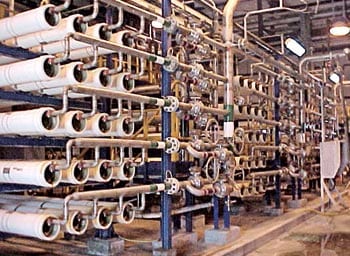
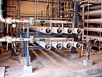
Entering the RO system, the treated and filtered seawater encounters three first-pass trains of high-flow seawater membrane elements (Figure 1) and two second-pass trains of low-pressure brackish water membrane elements (Figure 2) with very high salt rejection. Each first pass—consisting of a single array of 20 pressure vessels with seven elements per tube—has a capacity of 317 gpm and is rated at 42% recovery. Each second pass has a capacity of 143 gpm.
Part of the first-pass permeate is used for process water, following the addition of sodium hydroxide for pH correction. The rest of the permeate goes to a storage tank and is pumped through cartridge filters into the second pass, which consists of a 3:1 array of four pressure vessels with seven elements per vessel.
|
1. Removing the salt. The first pass of the reverse osmosis train cleans up seawater enough for use as plant process water. Courtesy: Koch Membrane Systems Inc.
|
|
2. Final cleanup. The second pass produces water clean enough for use as boiler makeup. Courtesy: Koch Membrane Systems Inc.
|
Working out the kinks
Water samples taken during the RO system’s commissioning indicated that the total hardness of the first-pass permeate was 16 mg/l (as CaCO3), with chloride at a 170 mg/l level. These values were in line with anticipated values. Over time, the feed pressure settled to less than 885 psi, which was better than anticipated. Following commissioning, the normalized flux level became relatively stable and remained so for about two years, after which it declined. During those first two years of operation, the normalized differential pressure across the system rose slowly from about 11.6 psia to 27.6 psia. Later, however, it rose more rapidly, to 47.8 psia.
Together, the decrease in flux level and the increase in differential pressure suggested that significant fouling had occurred. Records from 2002 indicate that the system’s feedwater had an SDI15 (15-minute silt density index) between 1 and 2. But by 2004, the feedwater SDI15 had deteriorated to between 4 and 5. The increased fouling and element blockage was attributed to a deterioration in feedwater quality. Despite regular cleaning, the blinding of the membrane and the blockage of the element feed channel could not be fully reversed. Initially, the system was cleaned every two to three months; later, the frequency was increased to monthly. Because it was thought that much of the fouling was due to biogrowth, sanitizing elements were added to the system.
The normalized salt passage of the system has remained stable over its service life. However, in the summer of 2004, seawater temperatures exceeded 86F—well above design values. Because conductivity rises with temperature, the quality of the system’s output could no longer meet plant requirements. A row of pressure vessels was taken off-line to improve the quality by increasing the flux.
Despite these problems, over its first five years of service the system generally has performed very well. The seawater elements have operated at lower-than-expected pressure, and both passes have been able to produce enough permeate of sufficient quality. Performance has been maintained by regular cleaning, with little deterioration in overall product water quality.
How to minimize DI operating costs
How much does it cost to operate the typical power plant demineralizer (water deionization) system? Few plants have a good handle on their fixed water treatment costs, much less the variable ones. During a recent Six Sigma project at a power plant, the costs of all consumables used by its demineralizers were studied for the purpose of developing strategies to minimize them. Table 1 summarizes the study’s findings.
|
Table 1. Breaking down the costs of demineralizer consumables Source: Recirculation Technologies Inc.
|

One of the most popular demineralizer system metrics is its efficiency, calculated as:
Total pounds of acid used per 1,000 gallons (net) of deionized (DI) water + Total pounds of caustic used per 1,000 gallons net DI
This metric, however, is useful only when acid and caustic prices are stable. When those prices fluctuate, a more-functional demin system metric is its cost efficiency, defined as:
Total cost of consumables (in dollars) per 1,000 gallons net DI
The "net" term in all three cases represents total DI water production, less the amount used for cation and anion regeneration. The reason that the second, cost-based expression is "better" is that it includes all the costs identified in Table 1. For the plant whose demin system variables are shown in the table, the cost efficiency worked out to $3,642.41 divided by 1,200,000 gallons, or $3.03/1,000 gallons net DI.
The power plant put this calculation of cost efficiency to very good use. Reviews of one year’s worth of data in the plant’s distributed control system and water treatment logs revealed a considerable number of "short" runs—runs in which the demin system was taken off-line early. Further statistical analysis quantified the negative impact of this poor operating practice: Over the year, the system’s cost efficiency was nearly $6/1,000 gallons, or a whopping 94% over the design basis. This got the attention of management, which immediately instituted a six-month corrective program, including increased operator training and resin cleaning.
Costs always rise
Once the basic operation of the demineralizer has been straightened out, other cost factors can be examined with an eye toward minimizing them. After several months of operation, as ion-exchange resins are depleted, the cost efficiency of any demin system—especially one that treats surface water—will inevitably increase. The positive slope of the curve in Figure 3 shows how significant the increase in operating costs can be. At the plant that conducted the Six Sigma project, once the cost efficiency hit $4.50, management again took notice and asked why the costs of the demin system were rising. The answer, according to engineers, was organic fouling of its resins.
|
3. Demineralizer cost efficiency. Detailed data collection is required to determine actual demineralizer costs. Source: Recirculation Technologies Inc.
|
Traditionally, power plants address slowly rising demin system operating costs in one of two ways:
- They tolerate the costs until operating costs exceed the cost of new resin. At this point, the fouled resin is replaced rather than thrown away (which would not be economically sensible). In plants that don’t closely monitor their demin plant costs, the reduction in service life becomes so great that the resins cannot be regenerated quickly enough to maintain the DI storage tank’s level. Rental demineralizers are called in to make up the shortfall. Only then are the resins changed out. Changing out resin before its true demise wastes money.
- Many demin plants replace resin far sooner than necessary. Cation resin should last, on average, in excess of 10 years. Strong base (Type 1) anion resins should last six or seven years. Before reliable cleaning options became available, however, replacing resin was the only viable way to return a failing DI plant to required production levels. Recirculation Technologies Inc. (Warminster, Pa.) endorses replacement of truly expired resin. But replacing resin years ahead of its expected demise cannot be justified when a less-costly (and more-effective) cleaning option is available.
When to clean
The best strategy for controlling demineralizer operating costs is to determine the optimum resin-cleaning frequency. It should be based on real cost data and include projections of resin life expectancies. Considerable savings can be realized by cleaning resin, as opposed to tossing it out. Increases in throughput alone can cut operating costs considerably.
Using typical operating costs, Recirculation Technologies has developed a new economic model for demin plant operations (Figure 4). As the graph indicates, by the beginning of Month 1 (following cleaning of its resins), the DI plant exhibited a 40% increase in throughput, lowering the monthly cost of operations by the same percentage. Several months of excellent (low-cost) operation ensued. Then, beginning in Month 6, the resins began to foul again due to accumulations of organics from raw inlet water, and operating costs began to slowly rise.
|
4. New DI economic model. Use these demineralizer operating cost curves to determine the best time to clean your anion resin. Source: Recirculation Technologies Inc.
|
From Month 6 onward, the model tracks the cumulative additional cost of operating with unclean resin. Recirculation Technologies suggests that the optimal time to clean the anion resin is when the cumulative additional cost has risen to match the cleaning cost. Why is that the optimal time? Because cleaning earlier costs the plant money in the form of savings not realized, and cleaning later costs the plant money in the form of operating costs over and above those of cleaning. Cleaning resets the cost curves back to Month 1—at a fraction of the cost of buying new resin.
New technology available
|
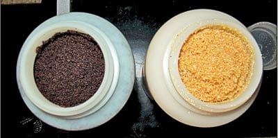
5. Chameleon resin. The same resin, before (left) and after cleaning with ReStore+. Courtesy: Recirculation Technologies Inc.
|
|
Table 2. Results of resin cleaning by ReStore+. Source: Recirculation Technologies Inc.
|
There used to be few options available for cleaning anion resins fouled with organics other than the use of brine and caustic. The "before and after" resin samples shown in Figure 5 show the effectiveness of a new process offered by Recirculation Technologies called ReStore+. It restores resins to golden, clear, almost new condition by removing 90% or more of fouling organics. As a result, demin system throughput usually doubles, cutting operating costs in half. Table 2 lists some results obtained to date.
Advanced flow meter works with shorter pipe runs
Four years ago, Finland’s Kvaerner Power Oy (with U.S. headquarters in Charlotte, N.C.) began a project to design and build the flue-gas treatment system for a new combined heat and power (CHP) plant being constructed by the Finnish utility Kotkan Energia Oy. The system’s most challenging spec: It had to fit in a specific, space-constrained section of the plant, which was designed to generate electricity as well as steam for district heating.
In this flue-gas treatment system (as in most others), liquid flow meters play a key role. They help to control the amount of water circulating through heat exchangers that extract energy from the exhaust of the plant’s boiler—in this case, a biofuel-fired unit. The circulating water also is used by the flue-gas treatment system to wash pollutants out of the boiler’s gas stream.
Engineers usually specify either conventional magnetic- or orifice-flow meters for such applications. For Kvaerner Power, the space constraints of the Kotkan plant effectively ruled out both technologies. Each requires the presence of long, straight, disturbance-free pipe runs upstream and downstream of the measurement device to smooth out the flow. Without these long runs, the flow of fluid at the meter would be too inconsistent to be measured 
precisely.
An unconventional solution
For the Kotkan project, Kvaerner Power ended up specifying a V-Cone flow meter from McCrometer Inc. (Hemet, Calif.). By manipulating differential pressure, the V-Cone conditions fluid flow, providing a stable flow profile that increases accuracy. A cone inside a tube at the center of the meter interacts with the fluid flowing through it, reshaping the velocity profile and creating a region of lower pressure immediately downstream.
The difference in pressure between this region and static line pressure can be measured by two pressure-sensing taps, one slightly upstream of the cone and the other in the downstream face of the cone itself. Plugging the reading into some form of the Bernoulli equation yields the rate of fluid flow.
The cone’s central position in the line optimizes the velocity of the liquid flow at the point of measurement. It forms very short vortices as the flow passes the cone. These short vortices create a low-amplitude, high-frequency signal that is very stable. This stability leads to highly stable flow profiles and repeatable flow measurements. Just as important from Kvaerner’s perspective, the V-Cone can do all this without long pipe runs on either side. The meter requires only that there be straight runs 3 diameters upstream and 1 diameter downstream of it.
|
6. Cone-powered. The V-Cone flow meter’s unique design allows it to accurately measure irregular fluid flows in a vertical orientation. Courtesy: Kvaerner Power Oy
|
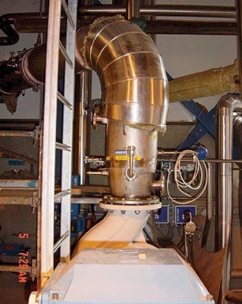
The cost of installing any technology either enhances or detracts from its inherent value. In the case of the Kotkan project, the selection of a V-Cone meter for the flue-gas conditioning system resulted in substantial avoided costs—of expensive, long lengths of upstream and downstream pipe that did not have to be purchased or installed. Kvaerner estimates that, including the cost of building a service platform for the flow meter (Figure 6), the choice of the V-Cone saved $13,750 on this job. The meter, which was installed during the spring of 2003, has reliably and accurately measured the flow of circulation water in the flue-gas system since then. The final installation included about two diameters of straight pipe upstream of the V-Cone and a 45-degree bend just downstream of the meter.
Why tubing beats piping
Plant engineers and technicians are having a tougher time building, maintaining, and upgrading the piping and tubing that interconnect plant systems. The performance expectations for piping and tubing are much higher than they were 10 years ago as a result of both stricter environmental standards and increased cost pressures. Many leaks that used to be considered nuisances now are classified as fugitive emissions or hazardous spills that can be costly to correct and may lead to a complete plant shutdown.
Although power plant economics and business models have changed, assembly and maintenance of piping and tubing have not. Pipe remains the material of choice for many plant applications, with flanges, fittings, and welds making connections in much the same way as they have for decades. However, the integrity of most piping systems depends on sealing and fastening techniques that were developed nearly a century ago. Today, many question whether traditional piping methods have kept pace with new industry requirements and cost consciousness. For many applications, tubing has emerged as a viable alternative to small-bore piping for two reasons: It is less prone to leaks, and it costs less to install.
Small line? Think tubing
Piping has traditionally been used where large fluid flows are required. However, tubing now is readily available in larger diameters and in a variety of wall thicknesses and materials. Generally speaking, tubing can replace piping in lines up to 2 inches in diameter. Pipe still should be used in lines more than 2 inches across.
Tubing has been used extensively and performed reliably in instrumentation systems with lines of 1/2-inch diameter or less. Here, tubing’s popularity comes from its ability to reduce system size and improve flow rates.
Tubing’s flexibility is another advantage over piping. Less energy is lost to the gradual bends and smooth inside diameter of tubes than to the sharp bends of pipes. Because tubing can be bent, it has fewer points of potential leakage than an equivalent run of pipe. Tubing’s ability to be bent at any angle is another plus. Because most pipes are bent only at 45 degrees or 90 degrees, more space is required to route them into a system.
It is a common misconception that bending a tube weakens it. In fact, the bend will usually be structurally stronger than a straight run, due to the hardening that accompanies bending.
Performance, cost advantages
Tubing systems can be built more quickly and inexpensively than piping systems because they need less equipment and far less labor per connection. Pipes are connected by welded, flanged, or threaded connections, whereas tubing is connected by fittings. Welding pipe is a labor-intensive process requiring highly skilled workers. Each pipe must be cut, prepped, aligned, and tack-welded. Each joint then must be finish-welded to complete the system. Tube fittings can be installed with standard wrenches, whereas pipe fittings may require threading or welding. In addition to weld consumables, installations of welded pipe may require hot work ("burn") permits, high-voltage electric power, additional personnel for compliance with OSHA "fire watch" rules, and other craft support.
Threaded connections may be simpler to make than welded connections, but they have their own problems. Field threading can produce threads of varying quality and finish, which can impact installation time and contribute to higher scrap rates. Sealing compounds or PTFE tape may have to be applied to reduce leakage. Nonetheless, sealed pipe joints that are subjected to extremes of temperature, pressure, or vibration aren’t immune to leaking over extended periods of time. A possible contributor to leakage is the pipe thread sealant itself, if it reacts with the fluid moving through the line.
Tubing, by contrast, is cut to length and deburred. Fittings are easy to install simply by tightening a nut that swages ferrules onto the tubing. The fitting creates a mechanical, metal-to-metal seal, producing a leak-tight connection. Some tube fittings can be gauged to ensure proper tightening before the system is pressurized and started. Tubing’s flexibility also enables systems to be aligned before any fittings are tightened, making it easier to reposition system components for maximum benefit. An example would be reorienting a gauge to make it easier to read.
If welding is the only or the preferred option, a tubing system installed with an orbital welding system can still outperform pipe. Compared with manual pipe welding systems, orbital welding systems—particularly those controlled by microprocessors—are quicker and more user-friendly. Their weld fittings are designed specifically for tubing, and the microprocessor ensures repeatability of welds and minimizes operator errors.
The following comparison of installation times for 1-inch connections underscores the potential savings (Figures 7 and 8):
- Welding of Schedule 40 pipe usually requires one hour, from cutting stage through alignment to making the weld. Threaded pipe connections require an average of 48 minutes to cut, thread, align, and seal.
- Tube connections require 12 minutes for cutting, prep, and assembly. Tubes with diameters larger than 1 inch require only another 5 minutes.
|
7. Laying pipe. Pipe typically relies on 45º and 90º elbows to route a system. Eliminating these fittings can speed assembly, reduce potential leak points, and improve flow characteristics. Source: Swagelok Co.
|
|
8. Tubular experience. Tubing provides a more compact system and fewer leak points than an equivalent run of pipe. Source: Swagelok Co.
|
All told, tube connections can cut installation time by more than 50%. There are many resources available, both in print and online, to help estimate the cost for all types of pipe and tube systems (begin by entering "plumbing estimating" into a web search engine). Bear in mind that the figures are only estimates; regional labor rates must be considered for more-accurate determinations of total installation cost.
Although there are many places within a plant where tubing can be used, the decision to use it must be consistent with applicable codes, standards and regulations, as well as the design practices and philosophy of the end user. The technical requirements of the application also should be considered, because not every piping system is a candidate for replacement by tubing.