Understanding Open-Channel Flow Equations for Hydro Applications

Chezy and Manning developed equations that are used to determine the average volumetric flowrate in open channels. This article explains a laboratory method that was developed and tested to further identify and quantify the parameters that make up the roughness coefficients of those equations. This method uses a hydraulic flume, and makes use of the technique of dimensional homogeneity and a new exponential form of an equation for instrument calibration.

Accurately measuring average velocities in channels or culverts with surfaces open to the atmosphere has been a challenge for centuries. The larger the flow cross-sectional area the greater the inaccuracy or uncertainty of measurement.

Open-channel flow is governed by the Froude relation, the ratio of inertial forces to gravitational forces. Thus, it was recognized early in the history of hydraulics that the formula for such average velocity would need to be a balance between gravity, causing the flow, and channel roughness, seeking to retard the flow. It was also recognized that any such formula would have to be for uniform flow, that is, for steady state flow, such that the water depth relative to the bottom of the waterway is a constant, or d(y)/dx = 0.

It is noted that in pipe or pressurized flow the word uniform has a different meaning. In that application, it means that the velocity profile has a constant velocity over the entire cross-section. On the other hand, open-channel hydraulics has no word for constant velocity over a cross-section. In this article, “normal” means the first of these two definitions, that is, steady state and constant depth. All units in this article are engineering units as commonly used in the U.S.

Equations Developed by Chezy and Manning

The first recognized and most lasting “resistance” formula for steady state, open-channel flow is credited to Antoine Chezy. He was tasked with determining the cross-section and calculating the discharge for the Paris water supply, and increasing its flowrate. He did so in 1768 by comparing flow conditions between two water courses, the Courpalet Canal and the Seine River. His resulting formula was published in his report on the Canal de l’Yvette as:

V_avg = C x R^1/2 x S^1/2

where V_avg is the average velocity in feet per second; C is Chezy’s factor of flow resistance in feet^1/2/sec; R is the hydraulic radius (the cross-sectional area divided by the wetted perimeter) in feet; and S is the slope, which is dimensionless. However, Chezy’s work received little attention until many years after his death.

In 1889, an Irishman named Robert Manning, who was Chief Engineer of Ireland’s Office of Public Works, presented a paper entitled “On the Flow of Water in Open Channels and Pipes.” Although his main interest appears to have been hydrology, he derived an average “resistance” formula for open channels from all the different resistance formulas published up to that time. In today’s format, this equation, which we’ll call Equation 1 for future reference, is:

V_avg = (1.486/n) x R^2/3 x S^1/2

where n is Manning’s roughness coefficient, which is the same numerically in either U.S. or metric dimensional systems. In the U.S. system, it has units of second/feet^1/3. If using metric units, the 1.486 is replaced by 1.0 and its units are second/meter^1/3.

Manning’s equation has been the most successful of all open-channel empirical equations, based on the resistance to flow and derived from observation. In fact, it is no exaggeration to say it is the cornerstone of today’s science of hydraulic engineering.

However, in the classic sense, both Chezy’s and Manning’s equations have several similar shortcomings. First, they do not have dimensional homogeneity, that is, the units on the left side are not the same as the units on the right side. Such equations are usually derived by experimentation or observation and quickly lose accuracy if extrapolated beyond their range of observation. It is known that Manning’s equation loses accuracy with very steep or shallow slopes. Secondly, to achieve dimensional homogeneity, their constants or coefficients are not pure numbers, but are artificially assigned units.

Furthermore, Manning’s equation suggests the average velocity is more sensitive to the hydraulic radius than to the slope. This really is an incompatibility, because the very nature of open-channel flow is a function of the slope component of gravity. The shape of the water passage, as calculated by the hydraulic radius, does exert an effect on the absolute roughness, but it is not a primary effect on the average velocity itself. The lower the hydraulic radius ratio, the greater the percentage of the flow that is in contact with the roughness of the boundaries.

Additionally, the very nature of the equations is a contradiction. The equations describe an average velocity that exists at a cross-section perpendicular to the flow. Such a cross-section has an infinitesimal thickness in the direction of flow, while the equations rely on coefficients that are referred to as “roughness coefficients.” But the effect of such roughness needs a finite length to exist—it cannot have an effect over an infinitesimal thickness. This means the roughness itself must act on some other parameter that can exist over an infinitesimal length to retard the flow velocity.

Theory Behind a Laboratory Experiment

The accuracies of both Chezy’s and Manning’s equations depend on the selection of their individual roughness coefficients. This is usually done by comparison with known similar streams or from a reference book of pictures of streams. However, in the article titled “Dimensionally Homogeneous Form of the Chezy and Manning Equations,” published by Hydro Review in April 2014, I proposed a new experimental method of determining the constituent parts that comprise these roughness coefficients.

To demonstrate the technique, I presented to a graduate class in Renewable Energy Engineering enrolled in the Hydraulic Laboratory course at the Oregon Institute of Technology (OIT) in Wilsonville, Oregon, an experiment designed to identify and quantify the components of the roughness coefficients. This experiment would concentrate on Manning’s equation, and was based on using the principle of dimensional homogeneity. The OIT graduate students who participated in this laboratory experiment were Joshua Couch, Cole Harrington, Karissa Hilsinger, Tai Huynh, Krystal Locke, William Perreira, Cullen Ryan, Pauloi Santos Vasconcelos Jr., Anurak Sitthiwong, and Asmitha Velivela.

First, two parameters were formed: H_v/S and R. H_v represents the velocity head, that is, H_v = (α x V_avg²) / (2 x g), where α is called the velocity head correction factor or the Coriolis factor. This multiplier represents the additional energy contained in either open-surface or closed-pressure flow that exists whenever a velocity profile is not constant over a cross-sectional area. This is because fluid energy is a function of the square of the velocity, and the sum of the squares in each fluid stream tube is greater than the square of the sum of the velocities in each stream tube.

Numerically α is always equal to or greater than one and is dimensionless. The slope or S could have appeared on either parametric side, but was assigned to the H_v parameter, because in hydraulics there is more than ample evidence that the average velocity is a function of the square root of the slope, that is, V_avg ≈ S^1/2. Then, a laboratory experiment was designed that would allow data to be obtained and plotted as H_v/S versus R, both of which have units of feet. Therefore, any resulting experimental equation should have dimensional homogeneity.

The units of H_v, from Bernoulli’s equation, are foot-pounds per pound or “specific energy,” but are still homogeneous with R, which has units of feet. It is to be noted that as R gets larger, the wetted perimeter (P) gets smaller relative to the area (A). This means frictional resistance to flow must get smaller, and therefore, the average velocity should get larger. In other words, a linear relation between H_v/S and R should have a positive slope.

Test Apparatus

A small tiltable-bed laboratory flume with a swimming pool recirculating pump, which one student had conveniently built the prior semester, was adapted for use. It was immediately evident that measuring the velocity head correction factor in such a small flume would be impossible. The best alternative was to only measure slope, average velocity, and water depth for critical and uniform flow.

At critical flow, where the Froude number is equal to one, the least hydraulic energy is contained for a given quantity of moving fluid. Consequently, there should not be any additional energy available to form a non-constant velocity profile and the velocity head correction factor should be near one. In addition, because the flume was short, the energy in the fluid entering the flume needed to be matched to the energy level desired for a given flowrate in the flume, so that uniform or steady state flow was immediately achieved.

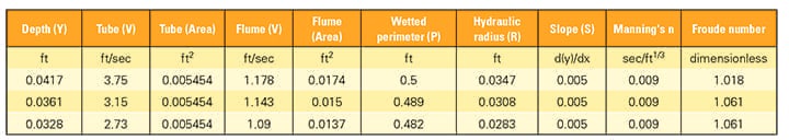
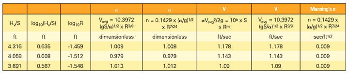
It was not possible to adjust the swimming pool pump that finely. Consequently, the team of researchers opted to bring in a second water tank, have the pump discharge into that tank, and then carefully siphon from that tank into the flume. A sonic flowmeter connected to the hose between the tank and flume gave the volumetric flowrate. It took a considerable amount of time and effort to get everything balanced for a single data point of steady state, uniform, and critical flow in such a small flume. However, ultimately three data points were collected, which were sufficient to demonstrate this method of data analysis (Tables 1 and 2).

Table 1.  This table shows data collected during three open-channel experiments conducted in the lab using a flume. Source: Lee H. Sheldon, PE

 

Table 2.  This table shows data collected during three open-channel experiments conducted in the lab using a flume. Source: Lee H. Sheldon, PE

It is emphasized these data points were closely spaced in terms of volumetric flowrate. This is because a five-inch-wide flume—operated for both uniform and critical flows—did not provide for a wide range of flow variability. Also, this experiment was done in a very smooth Plexiglas flume where Manning’s n was measured as only 0.009, whereas, 0.012 is the smoothest value in the published table of prototype water canals. Therefore, any numerical results should be viewed as applying only to this very narrow hydraulic regime.

However, it is also emphasized that the objective of this laboratory experiment was only to demonstrate whether this method could be used in future, more-extensive research to provide further insight and accuracy into the makeup of the components of Chezy’s and particularly Manning’s equations.

Data Reduction Technique

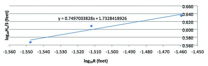
The plotting of these three data points was done in the same manner as the instrument calibration equation described in an article I wrote titled “A New Calibration Equation for the Winter-Kennedy Piezometer System,” which was published by Hydro Review in October 2013. This method yields a calibration equation directly in exponential form for ready comparison with the commonly used open-channel equations, that is, log₁₀(H_v/S) was plotted as the ordinate or y-axis and log₁₀R was plotted as the abscissa or x-axis (Figure 1).

1. This chart shows the model flume at critical and uniform flow. Source: Lee H. Sheldon, PE

These points closely approximated a straight line and yielded an equation of the form: y = mx + b.

log₁₀(H_v/S) = mlog₁₀R + b = log₁₀(R^m) + b

Raising both sides of the equation as powers of 10 yields:

10^(log₁₀H_v/S) = 10^(log₁₀R^m + b) = 10^b x 10^(log₁₀R^m)

Then, by logarithmic identity:

H_v/S = 10^b x R^m

or

H_v = 10^b x S x R^m

Substituting for H_v results in:

αV_avg²/2g = 10^b x S x R^m

Rearranging terms gives:

V_avg = (2g10^b/α)^1/2 x S^1/2 x R^m/2

Substituting numerical values of m = 0.7497 and b = 1.7328 from Figure 1 provides:

V_avg = (2g x 10^1.7328/α)^1/2 x S^1/2 x (R^0.7497)^1/2

It is noted that the slope (m) is positive as predicted earlier. Therefore:

V_avg = (108.1011g/α)^1/2 x S^1/2 x R^0.3749

Resulting in the following equation, which we’ll call Equation 2 for future reference:

V_avg = 10.3972(gS/α)^1/2 x R^3/8

Now, in this form, the open-channel equation contains only parameters that may be determined across an infinitely thin cross-sectional area. Comparing Equation 2 with Equation 1 provides insight into the relationships of the parameters in Manning’s equation.

V_avg = 10.3972 x (gS/α)^1/2 x R^3/8 = (1.486/n) x R^2/3 x S^1/2

Now, equating only the two expressions and canceling the S^1/2 terms gives:

10.3972 x (g/α)^1/2 x R^3/8 = (1.486/n) x R^2/3

Combining the R terms, results in:

10.3972 x (g/α)^1/2 = (1.486/n) x R^7/24

Which results in the following, which we’ll call Equation 3 for future reference:

= 0.1429 x (α/g)^1/2 x R^7/24

It is noted that Equation 2 does not have exact dimensional homogeneity. Neglecting the values of numerical coefficients, if the exponent of R had been 4/8 instead of 3/8, and with the inclusion of units for g (gravitational acceleration), it would have had exact homogeneity. Separately, it is noted that for Manning’s equation to have dimensional homogeneity, the units of n in Equation 1 had been historically assigned artificially as seconds/feet^1/3 or seconds/feet^8/24. In Equation 3, now, also including units for g, n has units of seconds/feet^5/24.

It is considered that these two differences in Manning’s equation and Manning’s n may be due to the uncertainty or inaccuracy of the data measurement in the limited test flume available to the students. Therefore, again, it is emphasized that the final numerical results of this experiment probably have a degree of uncertainty, but the method to more accurately quantify Manning’s equation is clearly demonstrated.

The term S(g) is the slope times gravitational acceleration. As the slope, d(y)/dx, becomes larger, there is a larger gravitational force acting to accelerate the flow.

As mentioned before, Manning’s equation is an average of all the open-channel equations published prior to 1889. The fact that it did not include the effect of the velocity head correction factor is quite understandable. It was not until as late as 1877 that the Coriolis velocity head correction factor was recognized to be a variable and not a constant.

The relationships of Equation 2 show Manning’s n is a metric for the velocity head correction factor, that is, n is proportional to α^1/2. Theoretically, if n is doubled, the velocity head correction factor is increased fourfold and the average velocity is halved. This is the mechanism through which the roughness of the fluid boundaries acts to retard the flow velocity across an infinitesimally thin cross-section.

As noted, Manning’s n is directly affected by the hydraulic radius (R^7/24). This does show that selecting a Manning’s n is not only a function of roughness, but of the cross-sectional shape of the water course. The fact that canals may exhibit some differences in Manning’s n due to their shape alone, as well as their roughness, has been previously documented in other literature.

In a paper titled “Determination of Rugosity Coefficient for Lined and Unlined Channels” published by the Karnataka Engineering Research Station in India, it says, “Flow in channels is complicated by the fact that the form of roughness elements and hence the resistance to flow are functions of the characteristics of channel shape and alignment. These factors make up the coefficient of rugosity or the roughness coefficient.” The reason, as mentioned before, is the smaller the hydraulic radius, the greater the relative percentage of the volume of flow that is in direct contact with the given absolute roughness of the boundary. Therefore, the greater the drag that the boundary imposes to retard the volumetric flowrate, the more non-uniform the velocity profile becomes, as calculated by α. Thus, the smaller the hydraulic radius, the greater the energy loss. Conversely, the greater the hydraulic radius, the more the velocity profile tends to become uniform over the cross-section. Coincidently, Chezy’s C is inversely proportional to R^1/8.

The equations developed by Chezy and Manning may appear to be very simple; however, they represent complex interactions of hydraulic parameters of fluids in open channels. The experimental process presented in this article may be used to study these interactions. The use of this experimental method, on the very limited and narrow basis described above, suggests that the difference between Chezy’s and Manning’s equations may not be as great as it appears. The real difference may be more in the degree of dependence that each coefficient of flow resistance has on the velocity head correction factor and the hydraulic radius.

—Lee H. Sheldon, PE is a hydropower engineer with 50 years of experience. He has published 33 technical papers and a college textbook on hydropower engineering, and has worked on every federal hydroelectric project in the Pacific Northwest, among others. He was formerly a professor at OIT, where he taught hydropower engineering and fluid mechanics.