What Is the Worth of 1 Btu/kWh of Heat Rate?

Decisions about design and operational options often are determined by one metric: the impact on the cost of electricity produced. An enhanced screening algorithm for power generation system total ownership cost (capital and operating) and thermal performance (output and efficiency) simplifies the analysis.

In a previous POWER article (“A More Accurate Way to Calculate the Cost of Electricity,” June 2011), traditional and expanded formulations of cost of electricity (COE) were discussed in detail. That article highlighted the pitfalls in using traditional formulas to analyze today’s highly flexible advanced combined cycle (CC) power plants. However, that analysis is valid only for very narrowly defined assumptions. This article will look into the same problem from a different perspective so that the analysis can be extended to all types of power generation problems.

The Apparent Value of Heat Rate

Using the basic COE formula and ignoring the change in operations and maintenance (O&M) costs, the maximum acceptable increase in capital cost (MACC) is calculated by equating before and after COE values for a given plant improvement (Equation 1).

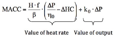Equation 1. Calculate maximum acceptable increase in capital cost (MACC). MACC is the capital cost equivalent of a given plant performance improvement (output and/or heat rate) with no change in cost of electricity. The parameters (in consistent units) are: H = annual operating hours; f = levelized fuel cost ($ per kWh in lower heating value in Equation 1, typically $/MMBtu in higher heating value); b = levelized carrying charge factor or cost of money; ∆P = change in plant net output (kW); ∆HC = change in plant heat consumption (kW in Equation 1, typically MMBtu/hr); h0 = plant net efficiency (base); and, k0 = plant-specific capital cost (base, $/kW).

The two components of the MACC formula give the value of plant heat rate (HR) or its equivalent efficiency(h) and output (P). In general, an improvement in CC heat rate (efficiency) comes with a change in output and heat (fuel) consumption (HC). If the improvement is limited to the bottoming cycle or combustion turbine (CT) hot gas path section, there is no change in CT heat consumption; that is, ∆HC = 0. This is the first “special case” explored below.

Using the well-known definition of efficiency and heat rate— h = P/HC and HR = 3,412/h Btu/kWh—it can be shown that the value of 1 Btu/kWh reduction in heat rate is given by Equation 2.

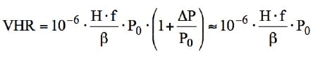Equation 2. Calculate the value of heat rate (VHR). The value of 1 Btu/kWh improvement in plant heat rate in dollars (VHR) is found using this equation. Note that P is in units of kW, f is in units of $/MMBtu (LHV), and P0 is the base value of plant output. Divide f by 293.071 to convert it to $ per kWh, used in Equation 1.

It is critical to use appropriate units and financial multipliers for the fuel cost in these calculations. Typically, fuel cost is quoted in dollars per MMBtu in higher heating value (HHV). For CC performance, on the other hand, the appropriate HR or efficiency measure is lower heating value (LHV). Furthermore, the most widely used metric in economic evaluations is the levelized COE (LCOE), which is obtained by multiplying the COE by a levelization factor (LF). LCOE provides a single number in current dollars accounting for the escalation of costs over the operational period of the power plant in question. For details, refer to “Cost Estimation Methodology for NETL Assessments of Power Plant Performance” published by the U.S. Department of Energy’s National Energy Technology Laboratory (NETL), available at http://tinyurl.com/bs874xl.

Thus, the fuel cost used in Equation 2 should be in units of $/MMBtu (LHV) and is found by f = f₀ · h · LF; where h = ratio of fuel HHV to LHV (1.109 for natural gas as 100% CH₄) and f₀ = base fuel cost in $ per MMBtu (HHV).

Appropriate values of LF and b can be obtained using formulas available in sources such as the NETL guide or the Electric Power Research Institute’s Technical Assessment Guide with pertinent economic assumptions and project financial structure. Representative values for independent power producer–owned CC plants with proven technology are 1.169 and 16% (levelized) for LF and b, respectively.

Alternatively, one can also calculate the value of one basis point improvement in net efficiency as a yardstick, as illustrated by Equation 3.

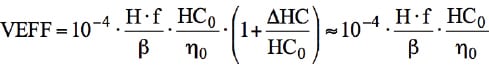Equation 3. Value of 1 basis point improvement in plant net efficiency in dollars (VEFF). LF and b are assumed as 1.169 and 16% (levelized), respectively. Note that HC is in units of MMBtu/hr and f in $/MMBtu, both LHV. HC0 is the base value of gas turbine (plant) fuel consumption. A basis point is one-hundredth of one percentage point, or 1/10,000.

Values of heat rate (VHR) and efficiency (VEFF) are plotted as a function of fuel cost in Figure 1. Two things should be noted in this figure. First, for F-Class technology, VHR and VEFF are nearly equivalent and can be used interchangeably. Second, for E-Class technology with lower efficiencies, VEFF is higher than VHR (which does not change with h₀). Furthermore, the difference is more pronounced at higher fuel costs. This is not surprising because the same incremental change (that is, one basis point) in efficiency is more valuable for older technologies burning a lot more fuel.

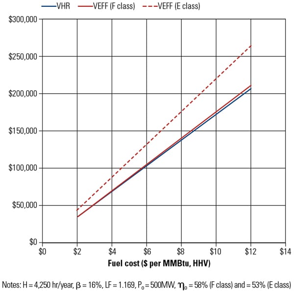1. Value of 1 Btu/kWh improvement in net CC heat rate (VHR) and 1 basis point improvement in net CC efficiency (VEFF). For advanced F-Class technology, VHR and VEFF are roughly equivalent. The values read from these curves can be scaled up or down for different values of H, b, LF, and P0 as needed. Source: Bechtel

Note that Figure 1 is a handy guide for determining the value of 1 Btu/kWh or 1 basis point of efficiency for different criteria. All one has to do is to scale the number read from Figure 1, as needed. In other words, for a CC plant using F-Class technology to be operated for 6,500 hours per year with $8 fuel, the value of each 1 Btu/kWh is (6,500/4,250) · $138K ~ $210K over the life of the project, expressed in current dollars. About the same value would be obtained for one basis point of efficiency.

The Intrinsic Value of Heat Rate

The numbers obtained from Figure 1 are probably familiar to some readers from personal experience. Unfortunately, for this special case with DHC = 0 (that is, efficiency/heat rate improvement is entirely due to bottoming cycle power output increase) the numbers from Figure 1 are also incorrect. As will be made clear in the following discussion, it overstates the value of heat rate by a very large margin.

In order to appreciate this, consider the second special case, where there is no change in CC plant output: DP = 0. In other words, efficiency/heat rate improvement is entirely due to reduced CT heat consumption. There are myriad ways to achieve this by optimizing the entire CT and/or CC system. A well-known example coming quite close to this special case is CT fuel heating (typically up to around 400F in modern F-Class units).

Algebraically, the resulting formulas for VHR and VEFF are the same as Equations 2 and 3. This, however, is counterintuitive. How can the value of heat rate be the same in two conflicting scenarios, one with a substantial reduction in fuel consumption and one with no fuel consumption reduction? Because there is no error in the mathematics, the answer is more philosophical, as the term “value” has nonmathematical connotations (recall the water/diamond value paradox—water is more valuable for life, but diamonds command a higher price).

The law of diminishing marginal utility best describes the concept. There is nothing wrong with improving CC plant efficiency with increased bottoming cycle output. In fact, this is the raison d’être for the combined cycle concept in the first place. A 300+ MW, 40% efficient system (a combustion turbine in simple cycle) is turned into a 500+ MW, 60% efficient system by the addition of a bottoming cycle. The value or utility of the additional 20 percentage points increase in net efficiency due to the additional 200+ MW is indisputable.

Not so clear-cut is the incremental value of the improvement or, in economic jargon, the marginal utility of the next 1-kW increase. In fact, the MACC formula in Equation 1 actually represents the marginal benefit of 1 kW additional CC plant output in terms of capital cost— DC/DP—which can be obtained by simply dividing both sides of Equation 1 by DP.

Special Case: Efficiency at Fixed Power Output. The divergence between pure mathematics and perceived value occurs when the marginal kW output has little or no value to the plant owner. Using the sample F-Class CC plant of Figure 1 with 500 MW and 58% thermal efficiency, assume that the designers come up with an improved steam turbine so that the net output increases 1%, to 505 MW. Because the CT is unchanged, fuel consumption remains unchanged, yet CC efficiency increases by 1%, to 58.58%. At $6/MMBtu fuel, the value of the additional 58 basis points in net efficiency is calculated as 58 x $105K ~ $6 million.

However, when this new technology is offered to the customer, the response is disappointing. From the customer’s perspective this is an unattractive value proposition because there is no need for the additional 5-MW output. In economic terms, the marginal utility of the extra 5 MW to that particular customer is zero. Because the additional 58 basis points in efficiency are tied to that output increase, its value is questionable, as the added output does not lower the customer’s fuel bill one single cent.

Fortunately, the indifference to additional output does not render the new technology valueless from a heat rate perspective. Figure 2 shows a typical CC part-load efficiency curve. The point labeled “Base” on the chart represents the old technology (500 MW, 58% thermal efficiency). The new base load point labeled “Improved” is 505 MW at 58.6%. Because the demand is for exactly 500 MW, the plant is run at 99% of full load with only 0.2% penalty in net efficiency (the point labeled “Corrected”). In other words, only 80% of the original efficiency improvement, which can only be achieved at base load, is realized. Thus, the heat rate or efficiency value calculated using the original formulas in Equations 2 and 3 should be reduced by 20%. This can be introduced into the formula by a multiplicative realization factor (RF).

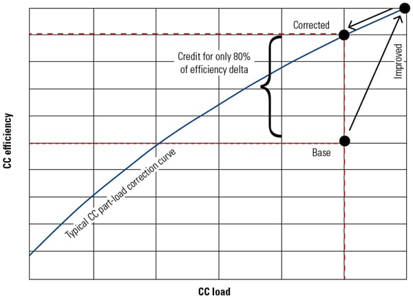2. Realization factor. The correction for CC efficiency improvement achieved by CC output increase only (with the same heat consumption) is the realization factor (RF). The shown RF (80%) is for a typical unfired CC part-load correction curve. For a specific unit the OEM-supplied curve should be used. Also note that the approximation is valid for ∆P/P0 of about 1% to 2%. Source: Bechtel

General Case: Value of Each Btu/kWh. Having found the answer for the specific case, the next step is to look at the general case, where 1% improvement in net plant output is accompanied by an arbitrary x% improvement in net efficiency. Realization factors have been calculated for a range of efficiency improvements accompanying 1% improvement in P by Equation 4.

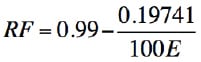Equation 4. Calculate realization factor (RF). The RF is applied to VHR and VEFF via the conceptual approach described in Figure 2. E is the efficiency improvement factor, which is defined as percent change in h per percent change in P.

As an illustration, consider the same sample 500-MW F-Class CC plant of Figure 1 with 58% thermal efficiency. Suppose the CT compressor is upgraded with new technology to give 0.7% higher CC output and 0.3% higher CC efficiency (new CC performance is 503.5 MW and 58.17%, respectively). What is the value of each basis point in efficiency for $6 fuel and 6,000 hours per year?

From Figure 1, at $6 fuel, each basis point is worth about $105K, which is scaled up for annual hours to (6,000/4,250) · $105K ~ $148K. The efficiency improvement factor E is 0.3/0.7/100 ~ 0.0043 (or 0.43% for each 1% in P) so that RF from Equation 4 is 0.53. Thus, the value of each basis point net CC efficiency increased for this CT compressor upgrade is 0.53 · 148K = $79K. This value is the intrinsic value of each Btu/kWh of CC net heat rate, which is completely independent of power output and produces a reduction in plant heat (fuel) consumption.

The More Rigorous Approach

Even after separating plant output and heat consumption effects to arrive at the intrinsic value of heat rate/efficiency improvements, there are still some deficiencies in the evaluation. The traditional LCOE formula does not account for many factors that affect field performance, operability, maintenance, and cost of generation over the economic life of the CC power plant, as was discussed in the June 2011 POWER article. Other factors of interest include annual site ambient and load variation, start-stop cycles, unrecoverable degradation, maintenance factors, reliability, emissions, and replacement costs (capacity and energy). A revised and expanded formula to account for all these factors was proposed in that article.

Although the new formula introduced in the earlier article is reasonably compact and easy to implement in a spreadsheet for rigorous evaluation of a cycling CC power plant, it does not lend itself to algebraic manipulation to arrive at simple formulas similar to Equations 2 and 3. Thus, in order to evaluate VHR or VEFF (while accounting for the effect of efficiency on plant emissions, maintenance factors, and reliability in a realistic operating scenario, including ambient and load variations) one should simply calculate LCOE for base and improved plants and find the allowable capital cost increase to set the difference between the two equal to zero. The key to the evaluation is to use the same kilowatt-hours of generation for base and improved LCOE calculations. The higher power output will be reflected in the capacity replacement term and the load factor, which determines the mean-effective plant efficiency, and appears in the fuel and emissions costs.

The earlier sample calculation (F-Class CC plant, 500 MW, 58% thermal efficiency, $6 fuel, and 6,000 operating hours per year) is updated for a typical cycling duty (with a capacity factor of ~50% and load factor of ~75%) at a site with annual average temperature of 65F; the assumptions are summarized in Table 1. Values of RF have been calculated for varying efficiency improvement factors, using the calculation procedure described in the previous paragraph. The results are shown in Figure 3.

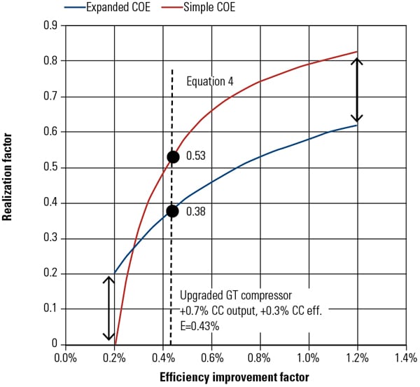3. Realization factors from Equation 4 and from the solution of equal-COE construction using the expanded COE formula. E is the efficiency improvement factor, which is defined as percentage change in h per percent change in P. Plant reliability, maintenance, and degradation factors are kept constant. Source: Bechtel

Two items of interest emerge from Figure 3. First, accounting for the real plant capacity factor (~50% instead of 6,000/8,760 = 68.5%) and load factor (~75% instead of base load) results in lower RF at high E and higher RF at low E. In other words, significant efficiency improvement at base load does not translate well into real operation at lower effective load factors. Second, modest efficiency improvement at base load is still modest at such low load factors, but it is not wiped out either. Revisiting the earlier CT compressor upgrade example, RF at E = 0.43% is 0.38 (instead of 0.53), so that the intrinsic value of each basis point net CC efficiency (or each Btu/kWh of CC net heat rate) for this CT compressor upgrade is 0.38 · 148K = $56K.

A Simple Rule of Thumb

Obviously, results will change if a certain improvement is expected to have a favorable (or, more likely, unfavorable) effect on overall plant reliability, maintainability, or performance degradation. Furthermore, only CO₂ emissions are considered here, and only at an assumed cost (see Table 1). Penalties associated with other emissions (such as NO_x emissions during startup) and their inclusion should also affect the final result. All these factors can be evaluated rigorously by the full application of the expanded COE model and underlying assumptions on a case-by-case basis.

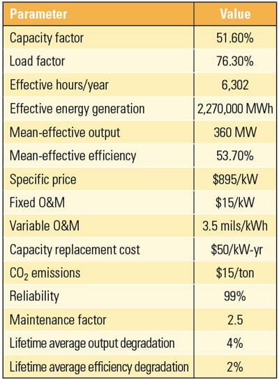Table 1. Parameters used in expanded COE formula. Data is partially taken from Table 1, “A More Useful Way of Calculating the Cost of Electricity,” June 2011. Source: Bechtel

For most up-front conceptual studies and back-of-the-envelope-type preliminary evaluations, discounting the heat rate value obtained from the original formula by the factors read from Figure 3 should be sufficient. In fact, for most practical purposes, just using a realization factor of 0.5 across the board is a good first-cut approximation to start the discussion on a given CC performance-cost trade-off topic.

– S.C. Gülen ([email protected]) is a principal engineer for Bechtel.