Business

A More Accurate Way to Calculate the Cost of Electricity

Life-cycle cost of ownership is a common metric used to compare power plant system alternatives. However, the familiar formula for calculating the cost of generating electricity omits factors that are becoming increasingly important to business decisions. A new formula addresses those blind spots by estimating the value of the part-load performance of cycling combined-cycle plants.

Previous articles proposed more accurate and consistent definitions of combined heat and power (CHP) efficiency (“A Proposed Definition of CHP Efficiency,” June 2010) and steam plant efficiency (“Plant Efficiency: Begin with the Right Definitions,” February 2010). This article proposes a revision of another common definition: the unit cost of generating electricity (COE). COE is a widely used metric for comparing power plant system alternatives. Traditionally, it combines a power generation system’s ownership costs (capital and operating) and thermal performance (output and efficiency). This metric is useful when comparing power generation alternatives that use similar technologies.

The standard formulation of COE is the sum of capital, fuel, and operations and maintenance (O&M) costs of plant ownership, as shown in Equation 1 (see sidebar).

The cost of generation as provided by this COE formula can be interpreted as the price at which electricity must be sold in order to cover all fixed and variable generating expenses and to match the return on company’s equity implicit in the assumed cost of money (ß). The COE is limited to a single operating condition, typically new and clean rated performance, and is usually calculated at International Organization for Standardization (ISO) baseload.

This definition of COE is useful for initial screening studies and comparison of baseload combined-cycle (CC) power plants. At this time, however, many CC units are relegated to daily cycling operation that entails frequent starts and stops as well as large load swings, often to provide spinning reserve and backup power for renewable energy generation that is not dispatchable. Even assuming that natural gas prices hold steady at their current low level, gas-fired CC plants are expected to continue in intermediate and cyclic duty for many years to come. Consequently, an overhaul of the standard COE formula is needed to determine the value added by improved operational flexibility, such as better part-load efficiency and faster starts.

Cyclical Operation

Typical daily operation of a “two-cycled” CC plant is shown in Figure 1. The plant is operated five days a week year-round or perhaps only during the summer months. In this example, every Friday, the plant is shut down at 10 p.m. for the weekend and is restarted the following Monday at 5 a.m. Twice a year, the plant is shut down for one week to carry out scheduled maintenance tasks. Thus, the annual plant start schedule comprises 250 starts (two cold, 48 warm, and 200 hot starts).

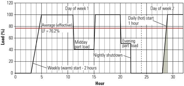1. Typical cyclical duty profile for a combined-cycle plant. This particular plant’s operation is sometimes described as “two-cycled.” Source: GE Energy

Ignoring the time spent during start-up (the added generation is estimated later) and the seasonal ambient variation, the plant is expected or planned to operate (H) 4,250 hours per year with a service factor (SF) of 4,250 / 8,760 = 48.5%. At a nominal 500 MW baseload power, the total annual energy production (E) can be calculated as 1,700,000 MWh for a capacity factor (CF) found as 1,700,000 / (500 x 8,760) = 38.8%. Similarly, the load factor (LF) is calculated as 1,700,000 / (500 x 4,250) = 80%, or nearly twice the CF.

Power generation during start-ups can be estimated via simple integration (see the shaded area in Figure 1 for a hot start) based on applicable start-up curves provided by the manufacturer. Using the load profile in Figure 1 and typical start-up curves, an additional 29,400 MWh per year of start-up electric generation is estimated.

Load ramps can be found in a similar fashion to contribute another 5,200 MWh, assuming a rate of 10% per minute. Adding these two unsteady-state generation quantities to the nominal generation of 1,700,000 MWh calculated above, you find the effective total generation (E_eff) is 1,734,600 MWh. Total or effective operating hours (H_eff) are higher than the nominal operating hours, H, by the total time spent during plant starts (shutdowns are ignored), or H_eff = 4,250 + 200 x 1 + 48 x 2 + 2 x 3 = 4,552 hours. This corresponds to an effective plant output (P_eff) of 1,734,600 / 4,552 = 381 MW. Thus, the correction due to the dynamic effects of start-up results in an effective load factor (LF_eff) of 381 / 500 = 76.2%.

Note how accounting for the energy generated during start-ups reduced the load factor by about four percentage points when the additional operating hours at low loads are included. This fact hints at a key advantage of fast-start plants that spend less time at low loads: the LF_eff and h_eff are higher, resulting in a favorable (lower) COE.

Average cycling plant load factors of 75% to 80% and the adverse impact of the time spent during plant starts (200 or even more per year for such units) suggest that an improvement could be made to the basic COE equation to account for plant cycling effects. In addition to accounting for the load factor variation just discussed, many other key plant operability considerations could be included in the COE formula. The following four key factors, when added to the basic COE equation, will produce a more accurate evaluation of real CC plant operation:

Seasonal temperature variation
Nonrecoverable performance degradation
Reliability (forced outage rate)
System (dispatch) considerations

The first two factors can be readily accounted for by calculating a corrected base performance. Ambient correction factors can be found from OEM-supplied curves using an appropriate annual load-weighted average temperature, which can be directly calculated using a seasonal temperature variation chart. (For most moderate climates, the deviation from the ISO value is less than ~5F.)

Average or mean-effective values of output and efficiency degradation factors can also be easily found from supplier-provided curves. Both corrections are multiplicative and less than unity in magnitude (unless the plant is located in an extremely cold site), so the net overall impact is higher COE via lower effective values of power output, energy production, and load factor.

The availability of CC power plants based on advanced combustion turbines is normally quite high: usually above 90% and often above 95%, especially for F-Class units operated in large fleets, even in cycling service. The reliability of these turbines can be taken into account by multiplying the total energy generation with an assumed reliability factor (R) of 99% (the complement of the forced outage rate).

Continuing with the example above, R x E_eff = 99% x 1,734,600 MWh = 1,717,250 MWh. The expected reduction in the unit service hours due to a less-than-perfect reliability is thus reflected in a reduction of the unit’s total energy generation and, consequently, the load factor. The reduction in the latter will manifest itself in lower effective plant efficiency and, as will be shown below, in higher costs associated with capacity and energy replacement. Even a small reduction in reliability (worth ~17,350 MWh for 1 percentage point in this example) can easily negate a perceived advantage in rated performance or operational flexibility.

A New Formula

These system interactions suggest a modified and expanded COE formula that tailors the original formula, adds emission costs, and adds system impact costs such as capacity and energy replacement during outages.

At this time, there is no industry-wide accepted method to convert specific plant emissions (that is, pounds of pollutants such as NO_x, SO_x, CO₂, unburned hydrocarbon, particulate matter, and so on per generated MWh) into cost. Nevertheless, emission costs (or penalties) can be added to the COE via a term comprising two new parameters: c_i (price/cost of pollutant i in terms of $/ton) and m_p,i(plant generation of pollutant i in tons/kWh). These terms can also be used to represent a cost of emissions during start-up. Although they are not a concern at baseload, CO emissions can be a problem when the unit is turned down, especially during plant starts when the unit spends a considerable amount of time at low loads.

The last new term added, system impact, accounts for the variation in effective total MWh generation and output (ignored by the standard formula) that must be provided when a deficiency in energy (kWh or MWh) must be made up by bringing another unit in the system online and/or when a deficiency in capacity (kW or MW) must be made up by purchasing firm capacity from neighboring systems. The COE analysis is adjusted to a common annual total energy generation basis using the following terms:

S_c = System replacement capacity cost ($/kW-yr)

S_e = System replacement energy cost ($/kWh)

âˆ†P = Capacity to be replaced (kW)

âˆ†E = Energy to be replaced (kWh)

For multiple unit comparisons, the alternative with highest total energy production can be selected as the basis to determine âˆ†P and âˆ†E. Energy replacement cost (S_e) is dependent on the makeup of the particular generating system, for which the alternatives are evaluated using COE. Note, however, that the economic dispatch principle requires using a variable generation cost at least equal to or higher than that of the units under consideration. Otherwise, the replacing unit would already be online and generating electricity.

Case Study

The new COE formulation’s contribution to the life-cycle cost analysis is best illustrated using an example. Consider a standard 500-MW CC plant (57.5% rated efficiency) described as Plant A. Two enhancements are planned for Plant A: improved part-load heat rate and a faster start-up and load ramp capability (assumed 50% shorter time). The new product that incorporates these improvements will be called Plant B. The remainder of the key plant parameters and assumptions used in this case study are summarized in Table 1. The beneficial impact of the planned improvements on the COE is conceptually explained in Figure 2.

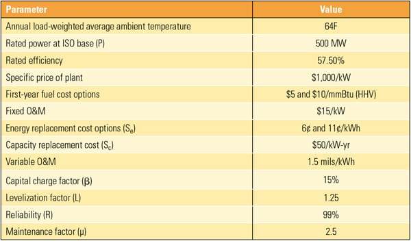Table 1. Key data and parameters used for calculating COE. The data shown here are for illustration purposes and do not reflect any existing product and/or guarantee. Sources: Electric Power Research Institute, U.S. Energy Information Administration, and PJM

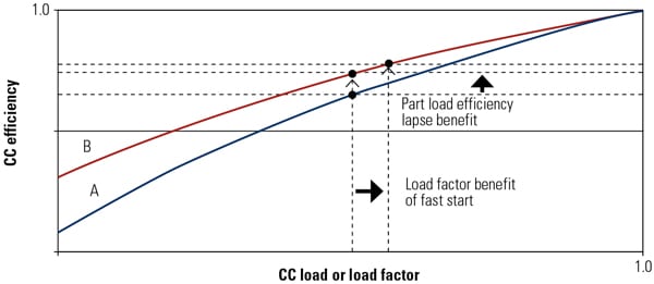2. Combined-cycle part-load efficiency. Plant B has better part-load efficiency lapse than Plant A in this hypothetical comparison. Thus, at the same average load, B has better efficiency (less fuel consumption) than A. The benefit of the faster start-up capability is a higher effective load factor (less time spent at lower loads) and, consequently, higher efficiency. Note that the generic curves shown here are for illustration purposes and do not reflect any existing product and/or guarantee. Source: GE Energy

Two operating scenarios for Plant B could be analyzed:

Scenario B1. Plant B reaches baseload quicker than Plant A, allowing the plant to be dispatched for a longer period. Therefore, it generates more revenue—but at the expense of higher total fuel consumption and emissions. H_eff is the same as for Plant A, or 4,552 hours (calculated previously).
Scenario B2. Plant B starts later than Plant A and reaches baseload at the same time as Plant A normally would. The benefit to operating in this manner is lower fuel consumption and emissions—but at the expense of less generation (less revenue). H_eff is reduced by 150 hours to 4,402 hours.

It would seem that starting a “fast” power plant as early as possible so that it contributes baseload power to the grid quicker (scenario B1) is a better strategy than starting it as late as possible to be online at the last minute (scenario B2). However, this may not be the case when electricity sale prices are taken into account.

If the price before the prescribed time when the market price becomes effective is significantly lower (or even below the variable cost of generation), the apparent advantage of B1 may be much more modest or even nonexistent. In fact, B1 is most likely to occur in an emergency situation, when immediate dispatch is required to exploit an opportunity or to make up for a sudden or imminent loss in generation.

However, B2 is probably the norm for regular plant starts. Furthermore, a plant may have fast-start capability, but the plant owner may choose to use it sparingly or not at all unless paid a premium by a system operator to dispatch on short notice at a significant premium. Thus, the actual value of the fast-start capability is more likely to fall somewhere between the two scenarios. For this example, a weighted average of the performance of the two scenarios is used.

A comparison of the COE calculated using the standard (original) and modified (proposed) formulations is shown in Figure 3. The new formulation returns a 25% higher value, driven by the use of “real” effective kWh and efficiency values (lower than their nominal baseload counterparts) and additional cost components. (Note the significant contribution of emissions even when only CO₂is considered. When NO_x, CO, and other emissions are also thrown into the mix with system-specific “known” costs, the impact will be more pronounced.) The real benefit of the proposed formulation, however, is its ability to account for plant metrics other than rated performance, thereby providing an improved plant life-cycle cost evaluation.

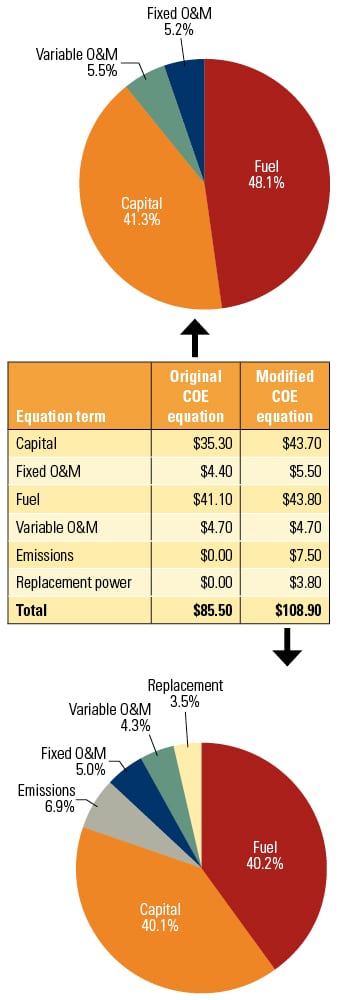3. Calculating the COE. Applying the assumptions listed in Table 1 to the original and modified COE formulas to Plant A illustrates the usefulness of this new way of calculating COE. The assumed price of natural gas used to calculate the COE was $5/mmBtu. An energy replacement cost of $60/MWh was assumed. Values shown in the table are in millions of dollars. Source: GE Energy

From the equipment supplier’s point of view, an interesting question is now raised: What is the market value of the Plant B upgrades, assuming Plant B COE remains the same as Plant A’s? If the Plant B upgrades are evaluated by assuming 10% unplanned starts (a reasonable assumption given the earlier discussion), then the results, summarized in Table 2, are quite interesting:

A CC design with a better part-load heat rate has a value of $7 million to $13 million for $5 and $10 fuel, respectively. This is quite significant when you consider that each 0.1 percentage point in rated efficiency is worth ~$1 million to ~$2 million (with the assumptions of this example) for the same fuel price range. The implication is that there is room for about 0.7 net CC efficiency points for a trade-off between ultimate rated performance and sustained performance across a wider load range.
A nimbler CC design, which slashes the start time and load ramp rate by 50%, has an additional value of $10 million to $13 million for $5 and $10 fuel for a total value of $17 million to $26 million compared with Plant A, assuming no difference in plant reliability, maintainability, or component degradation.
A reduction of 1% in reliability (R = 98% instead of 99%) is more than enough to wipe out all the value compared with Plant A, or even more (a reduction in value by $15 million to $22 million). The economics worsen if any potentially adverse impact on maintenance factor and/or nonrecoverable degradation is thrown into the mix.
In order to simplify the treatment herein, NO_x and CO emissions (typically reduced during faster starts) are ignored. Inclusion of either will increase the value of Plant B with the fast-start feature.
Similarly, in extremely hot climates and/or applications with duct firing, hot day part-load performance characteristics of the plant become important. This refinement can be easily incorporated into the proposed COE formula using applicable correction curves or a load profile table.

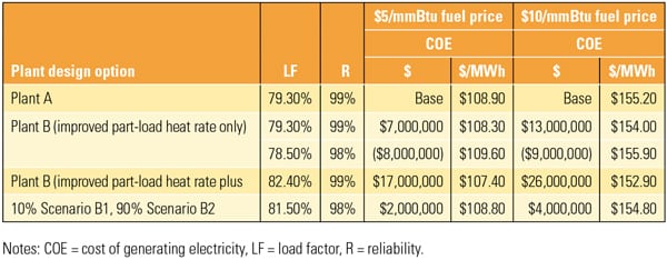Table 2. Evaluating the COE of two plant design options. Note the dramatic negative economic impact of a small decrease in Plant B’s reliability. The detrimental impact on plant economics would be even more pronounced should a maintenance factor and/or nonrecoverable performance degradation be considered as well. Dollar values reflect the difference from the Plant A baseline. Be aware that electricity sale price or ancillary market opportunities and payments are not included in this analysis. Source: GE Power

The expected increased use of CC plants in the future will place a premium on units that can be heavily cycled and quickly started. By adding these effects to the familiar COE equation, we get a new formulation that can be easily used to perform screening studies to determine the value of a plant more comprehensively.

In most applications, significant life-cycle cost savings are possible for plants that can operate at part load with improved efficiency or that can start and reach baseload faster than conventional plants. Now you have a screening tool to estimate the value of those operational improvements.

— S. Can Gülen, PhD, PE ([email protected]) is a principal engineer with GE Energy.