Strategies to Reduce Sulfuric Acid Usage in Evaporative Cooling Water Systems
Concentrated sulfuric acid is often used to prevent calcium-based scale formation on condenser and heat exchanger tube surfaces in power plant evaporative cooling water systems. Unfortunately, the chemical’s price has jumped more than 300% over the past three years. If the rising cost of water treatment has you under the budget gun, here are some alternative strategies that can reduce or even eliminate your sulfuric acid usage.
Sulfuric acid (H2SO4) can be the single largest chemical by volume used by power plants that have evaporative cooling water systems. Dramatic increases in the price of concentrated H2SO4 over the past few years have put a dent in the operation and maintenance budget for every plant that uses the chemical for pH control.
Price increases followed increased domestic and international demand while H2SO4 supply has decreased or, at best, remained static because of supply disruptions caused by hurricanes, shipping issues, and decreasing imports. In addition, the sulfur content in oil production has been lower than anticipated. Refineries used to pay to get rid of sulfur, but now many sell the product. H2SO4 prices averaged $50 to $100 per ton from 2005 to 2007 but increased significantly in 2008, when many plants paid $300 to $400 per ton. Some plants couldn’t get acid at any price — the chemical just wasn’t available.
Recently, the global economic slowdown has mitigated demand for the chemical somewhat, but price volatility and supply issues are expected to continue. As a result, proactive utilities are responding with programs to minimize or eliminate H2SO4 use in cooling towers. Before we discuss ways to minimize H2SO4 use, let’s begin with the several technical and operational challenges that any H2SO4 reduction program must address.
How High Is High?
The two most common questions asked about chemical usage in cooling towers are: "How high can I run my cooling tower pH?" and "How much money can I save?" There aren’t any closed-form solutions to these questions, but there is a process to follow that will result in useful answers. A typical acid reduction project consists of the following steps:
-
Create or validate pH/alkalinity model.
-
Perform mineral solubility analysis.
-
Modify or validate chemical treatment program.
-
Determine operating window.
-
Determine and mitigate risks.
The savings potential is necessarily plant specific. It depends on a host of factors, including the concentration of scale-forming minerals (primarily calcium and alkalinity) in the makeup water, the current pH target, and the cycles of concentration or alkalinity concentration in the cooling water. In general, acid savings are greater for cooling towers operating at lower cycles of concentration. Potential acid savings decrease at higher cycles of concentration because more acid is required to neutralize alkalinity that would otherwise concentrate.
Acid — The Alkalinity Destroyer
It’s important to understand the role that the acid plays in controlling pH, and that requires a basic understanding of the relationship between pH and alkalinity.
Alkalinity occurs naturally and enters the cooling water with the makeup water, regardless of source. Alkalinity remains in the water, and its concentration increases as evaporation occurs. Increasing alkalinity increases pH. Carbonate and other scales can form more readily as pH and alkalinity increase. Figure 1 shows the relationship between M-alkalinity or total alkalinity and pH. The curve in the figure is commonly used in modeling cooling tower performance, but it’s not consistent across all cooling systems. Any H2SO4 reduction program must begin with an accurate model of the pH/alkalinity relationship in the particular cooling system.
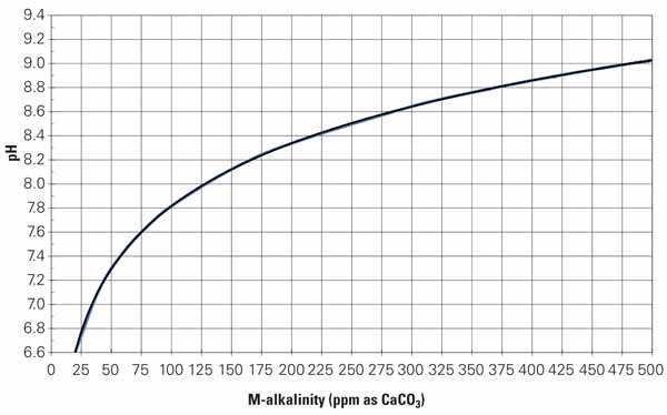
1. Develop custom curves. This typical M-alkalinity curve is commonly part of chemistry models used to determine the amount of acid needed to maintain a prescribed evaporative cooling water pH. The first step in any acid reduction program is to analyze water samples from your plant to develop your particular M-alkalinity curve. Source: Daniel Sampson
The M-alkalinity measurement is simply an acid titration — acid is added to a water sample until the pH is reduced to approximately 4.3 (the M-alkalinity endpoint). As such, the M-alkalinity measurement tells us the total alkalinity in the sample. This total alkalinity may be present in several different forms. Figure 2 shows a curve similar to Figure 1 but describes the relationship between the different alkalinity species as pH changes. At higher pH we see carbonate and bicarbonate alkalinity. We convert these forms into carbon dioxide (CO2) as pH lowers through acid addition. The free CO2 formed is scrubbed into the atmosphere as cooling water recirculates through the tower. H2SO4 destroys alkalinity by liberating CO2 to the atmosphere, defined by the following two chemical equations:
H2SO4 + Na2CO3 → H2O + CO2 → + Na2SO4 (destruction of carbonate alkalinity)
H2SO4 + 2NaHCO3 → 2H2O + CO2 → + Na2SO4 (destruction of bicarbonate alkalinity)
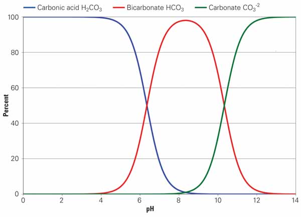
2. Finding normal relationships. These curves, related to Figure 1, describe the relationship between the different alkalinity species as pH changes. The higher pH results in carbonate and bicarbonate alkalinity that is then converted to CO2 as the pH is lowered through acid addition. Free CO2 formed is then scrubbed and released to the atmosphere as cooling water is recirculated and evaporated in the cooling tower. In sum, acid destroys alkalinity by liberating CO2 to the atmosphere. Source: Daniel Sampson
The amount of acid we need is directly proportional to the amount of alkalinity we want to neutralize, and that depends on the pH we want in the recirculating cooling water. It would be nice to simply shut off the acid feed and run the cooling tower at higher pH (and higher alkalinity). Unfortunately, scaling tendency increases with pH, so it’s not quite that easy. Some plants have also experimented with CO2 as an acid replacement (see sidebar).
Why Not Use CO2 as an Acid Replacement?
Many plants have attempted to replace H2SO4 with CO2. That can work, but it’s important to understand the limitations of CO2 when using it for pH adjustment.
Injecting CO2 into cooling water temporarily shifts carbonate alkalinity to bicarbonate as pH is lowered by the formation of carbonic acid. This does work at the lower pH circulating water, but the CO2 that’s liberated is stripped in the cooling tower. Therefore, cooling water pH returns to equilibrium as the water drops through the cooling tower fill and theCO 2 is released. Stripping the CO2 from the cooling water limits its usefulness for pH control. Tower M-alkalinity stays the same (Figure 3).
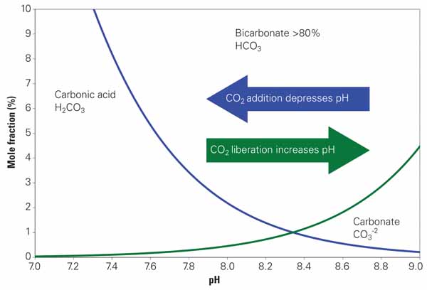
3. CO2 injection doesn’t replace acid. Sulfuric acid destroys M-alkalinity by liberating CO2 to the atmosphere. CO2 injection, on the other hand, temporarily shifts carbonate to bicarbonate as pH is lowered by the formation of carbonic acid. However, the CO2 is stripped in the cooling tower, returning pH to tower equilibrium with the M-alkalinity remaining unchanged. Source: Dan Sampson
CO2 injection points are critical. The gas must be injected into the circulating water after the water leaves the tower. CO2 can be injected into the discharge side of the cooling tower circulating water pumps or into the cooling water supply header just before the condenser. In either case theCO 2 can lower the pH in the pipes and condenser, but pH will again increase when the water passes through the tower. CO2 can be used to protect the condenser, but pH of the cooling water passing through the tower fill and in the tower basin cannot be adjusted, and scale formation may result.
Several alkalinity models exist, however, and selection of the "best" pH/alkalinity model should not be taken lightly. Different models will also produce different results (Figure 4), as small differences in the predicted relationship between pH and alkalinity can have significant impact in terms of potential acid usage. Good predictive data are critical, so develop pH/alkalinity curves specific to the water used at your plant. Developing specific curves requires only a few (from two to four) pH/alkalinity data pairs that can then be used to adjust the theoretical curves to reflect real plant conditions.
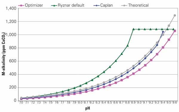
4. There are differences. Different pH/alkalinity prediction models provide different results. Analyze samples from your cooling water system to select the best model or correct one of the models to reflect your actual operating conditions. Source: Daniel Sampson
Table 1 analyzes potential acid savings by comparing normal and high pH cooling tower operation for different cycles of concentration for an example cooling tower. Although the limits change depending on tower operation and chemistry, the process for determining limits is common to any acid reduction project.

Table 1. Example calculations used to determine the effects of reducing acid on cooling water pH and M-alkalinity. The area highlighted in red indicates the “No Go” zone—the point above which scale formation will occur. A separate mineral solubility analysis (discussed in the next section) performed for this example indicates that scale formation will occur if M-alkalinity exceeds 400 ppm. Source: Daniel Sampson
In this example, the maximum allowable M-alkalinity was set at 375 ppm to provide some protection from transients based on the mineral solubility analysis. The "normal pH operation" cases shown in the table assume tower operation at a pH setpoint of 7.65 and an M-alkalinity of approximately 80 ppm. The "high pH operation" cases limit M-alkalinity to 375 ppm with a corresponding pH of approximately 8.8. At very low cycles of concentration (three cycles or less), no H2SO4 feed is required and M-alkalinity is naturally less than the 375 ppm limit. The need for H2SO4 feed increases as cycles increase, and potential savings decrease as cycles increase due to the concentration of makeup alkalinity in the tower circulating water.
For this mode of operation, the increase in pH allows an increase in alkalinity and a reduction in H2SO4 feed equal to the increase in alkalinity. From Figure 1, a pH increase from 7.65 to 8.81 equates to 295 ppm of alkalinity increase, which is also equal to 295 ppm of acid use reduction.
Allowing an increase in pH can have a dramatic impact on the cost of plant chemicals. Table 2 shows the impact on H2SO4 usage in pounds and dollars for another scenario, where the tower is operated at four cycles of concentration with an M-alkalinity increase in the cooling water from 80 to 375 ppm. Acid usage was lowered by approximately 92%, reducing the cost of purchased acid by approximately $210,000 per year.
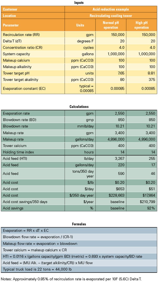
Table 2. Model your cooling tower chemistry. There are many available computer programs that model the cooling tower water treatment systems. This model will give the user an estimate of the reduction in acid purchases when operating at a high cooling water pH. While acid purchases may be reduced at higher pH, other chemical purchases may increase. Source: NALCO
The Need for Mineral Solubility Analysis
Detailed mineral solubility analysis is critical before any plant attempts to minimize H2SO4 use. Simply increasing pH is an invitation to disaster — or at least a badly scaled condenser. There are many mineral solubility programs available in the marketplace, and most specialty chemical suppliers have been trained in their use. Mineral solubility and corrosion modeling software evaluates the risk associated with corrosion, scale, and microbial growth based on makeup water chemistry, cycles of concentration, pH, and product dosage. Plant personnel must either educate themselves or get expert advice before attempting to minimize acid usage.
The willingness to accept additional risk is an important component of an acid reduction program. Any increase in pH or alkalinity carries an increased risk of mineral scale formation. Plants can mitigate risk through automation. Redundant pH analyzers, for example, can minimize the potential for high pH transients. Similarly, changes in acid feed systems to include variable-speed and redundant pumps can improve pH control and minimize risk further.
Mineral solubility analysis has an important role to play in mitigating the risk of scale forming on plant equipment. The analysis should be performed routinely as a part of the plant’s water-monitoring program to ensure that the treatment program and operating limits continue to provide adequate equipment protection to the cooling tower, condenser, and other components.
Chemical Treatment Programs
A chemical treatment program designed to work at the lower pH scale probably won’t work as pH increases. Mineral solubility analysis again can help. Specialty chemical suppliers should know what type of equipment scaling their products can inhibit and, more importantly, the point at which those same scale inhibitors will fail. These specific product capabilities must be included in the mineral solubility analysis.
In general, operation at higher pH requires significant changes in the plant’s water treatment program. Bleach, for example, may work well at lower pH, but it loses its ability to control microbial growth at higher pH, and bromine compounds may be required. General corrosion rates tend to be reduced as pH increases, but traditional corrosion control chemistries (like phosphate) may increase the risk of scale formation. Finally, the efficacy of scale and deposit inhibitors is highly pH dependent. A product that works well at lower pH may work poorly or not at all as pH increases. Also, new scale inhibitors may be required to stabilize scales that don’t form at lower pH. Some examples follow.
Calcium Carbonate Scale Inhibition. Lowering acid usage results in higher alkalinity and an increased carbonate scale-forming potential in the circulating water. The driving force is a function of calcium, alkalinity, pH, and temperature. Each of these variables influences the calcite saturation index (CSI), another measure of equipment scaling. Individual scale inhibitors exhibit different capabilities for preventing calcium carbonate scale. HEDP (a proprietary scale inhibitor), for example, can usually inhibit calcium carbonate scale up to a CSI of about 90. PBTC is a more effective nonproprietary calcium carbonate scale inhibitor than HEDP and can inhibit formation up to a CSI of about 120. The mineral solubility program used may include several of the common scale inhibitors. In any case, it’s best to work with a specialist to create a chemical treatment program.
Noncarbonate Scale Inhibition. Calcium phosphate exhibits decreasing solubility with increasing pH, especially above a pH of approximately 8.2. Effective calcium phosphate scale inhibitors must be used if phosphate treatment is to continue. Plants may consider nonphosphate corrosion control programs. The use of zinc, for example, may be useful if conditions allow it.
Silica must also be considered as a scale inhibitor. Silica exists as silicate ion at pH <8.4. Magnesium silicate formation may be a problem at higher pH. Best practice for predicting magnesium silicate scale formation is to carefully monitor cycles of concentration based on soluble constituents and compare this value to cycles of concentration calculated by silica. Careful monitoring is essential. If silica cycles are consistently lower, then silica precipitation (in various forms) may be occurring. Silica scale inhibitors do exist and can be used effectively, but there’s little experience with these chemicals at higher pH (>8.4). Again, careful monitoring is essential.
Corrosion Control at High pH. Corrosion tendency is normally lower as pH increases. High-pH operation may eliminate the need for phosphate-based corrosion inhibitors. Online corrosion rate measurement should be used to determine the need for active corrosion inhibitors. If active corrosion inhibitors are required, phosphonates can be used as cathodic corrosion inhibitors with alkalinity serving as the anodic corrosion inhibitor. As mentioned earlier, zinc can also be used as a supplemental cathodic inhibitor. Phosphonates may experience some reversion to ortho-phosphate, however, and increase the risk of calcium phosphate scale formation.
Begin with a good monitoring program that includes both corrosion coupons and online analyzers. Passive inhibition alone may provide acceptable corrosion control, especially if the cooling system contains little exposed mild steel. Again, alkalinity acts as the anodic corrosion inhibitor. A good active corrosion inhibitor should maintain a mild steel corrosion rate less than 3 mils/year (mpy) while acceptable results on a passive program would probably be in the 3 to 5 mpy range.
Copper alloy corrosion tendency lowers as pH increases. Azoles remain effective, and it may be possible to achieve good results at lower chemical feed rates.
Automate Your Cooling Tower
Minimizing acid usage requires higher pH and increases risk. Manual control of cooling tower chemistry increases this risk. Using online analyzers and monitoring tools can significantly mitigate the risk of scaling up your equipment. Specifically, the following online analyzers should be part of the cooling system monitoring program:
-
pH
-
Specific conductivity
-
Turbidity
-
Oxidation/reduction potential
-
Microbiological activity
-
Corrosion rates (specific to cooling system metallurgy)
-
Total dispersant feed
-
Dispersant residual
-
Dispersant consumption
-
Scale formation (using a heated element)
These instruments provide information on those key performance indicators that can quickly determine cooling system scaling, deposition, and corrosion potential. Information on dispersant feed and consumption is especially important. An increase in dispersant consumption, for example, provides a leading indicator for scale formation or deposition. It should be used to automatically adjust chemical feeds as required to maintain acceptable deposit and scale control. Likewise, online corrosion rate analysis allows rapid adjustment of the treatment program before damage occurs. Corrosion coupons should also be used, but they can only quantify corrosion after it has occurred.
A Case History
A nuclear plant with a pressurized water reactor wished to minimize sulfate concentration in the steam cycle. The premise was that minimizing sulfate in the cooling tower would result in less sulfate ingress to the secondary system. The expected payback included shortened chemistry holds during start-up due to lower sulfate levels, steam generator life extension due to fewer impurities, fewer acid trucks to unload, and a safety improvement associated with handling less acid.
Sulfate in cooling towers averaged 700 to 800 ppm and came from two sources. Some sulfate entered the cooling system with the makeup water (approximately 40 ppm) and cycled approximately 3.5 times to provide a cooling water sulfate level of approximately 140 ppm. The majority of sulfate came from acid addition (approximately 500 to 600 ppm).
The study evaluated several solutions, including the use of other acids, minimizing cycles of concentration (to reduce the sulfate contribution from the makeup water), and increasing pH (to minimize sulfate contribution from the acid feed). The use of other acids wasn’t practical, so the focus shifted to the other two water treatment alternatives.
Modeling and Mineral Solubility Analysis. The pH/alkalinity relationship was validated using existing plant data. The pH/alkalinity pairs were plotted and curve fitting was used to establish the relationship. Modeling indicated that pH could be safely increased from 8.4 to 8.8 and cooling tower cycles of concentration could be reduced to 2.45. Sulfate concentration in the cooling tower would lower to approximately 300 ppm (at least a 50% reduction). Modeling also predicted a substantial decrease in acid handling — about a 48% reduction in the number of acid trucks and subsequent deliveries.
The modeling included several scenarios. The preferred solution minimized acid usage and sulfate contribution. Specialty chemical costs increased, but H2SO4 costs decreased, and this solution was essentially cost-neutral.
A pilot cooling tower study provided confirmation of the modeling results. Cycles of concentration were set at 2.5 with a pH control setpoint of 8.8. The scale inhibitor was changed from HEDP to PBTC to provide additional calcium carbonate scale inhibition. The zinc-phosphate corrosion inhibitor was eliminated.
The pilot cooling tower study indicated no scale present on heat exchanger tubes. Corrosion rates were low (<2 mpy mild steel and <0.1 mpy copper nickel and stainless steel). Acid consumption and sulfate both dropped by approximately 50%, and there were no microbiological control issues.
The plant achieved other performance improvements: reduced sulfate in the cooling tower blowdown, less accumulation of mud and silt (because of operating at lower cycles of concentration), and significant reductions in both zinc and phosphate in the cooling tower blowdown. The reduction of sulfate, zinc, and phosphate in the blowdown were especially advantageous because the plant discharges directly to a river.
Identifying and Mitigating Risks. The acid reduction program increased the risk of scale formation (by operating at a higher pH) and also increased the risk of a National Pollutant Discharge Elimination System violation under the Clean Water Act, as the proposed operating pH (8.8) was closer to the plant’s discharge limit of 9.0.
The risk of scale formation was mitigated in several ways. Changes to the cooling tower chemical treatment program included automatic feed of a more powerful calcium carbonate scale inhibitor. Automatic feed was based on consumption; the controller can sense the onset of scaling and react immediately with increased dispersant feed. Alarm functions and an online deposit monitor were also added to the instrumentation suite.
The risk of a pH violation necessitated a thorough design review of the acid feed system. The review concluded that the existing acid feed system was sufficiently reliable. It was gravity-based (no pumps), included two separate systems, and had operated for 20 years with an availability of >99%. Additional pH alarm functions were added, and the calibration frequency of the five existing pH analyzers was increased. Finally, operating at lower cycles of concentration provided a slower rise in both alkalinity and pH in the unlikely event of a loss of acid feed.
With mitigation measures in place, the plant initiated a trial. Data after six months of operation confirmed findings from both the modeling and pilot cooling tower testing. Cooling water pH averaged 8.70 to 8.75 at 2.2 to 2.7 cycles of concentration. Makeup water alkalinity averaged 250 to 270 ppm with cooling water alkalinity of 400 to 450 ppm. The reduced cycles of concentration led to higher concentrations of active polymer (from about 1.5 ppm to an average over 3 ppm). Zinc corrosion inhibitor has not been needed to achieve acceptable corrosion rates (between 1.0 and 2.0 mpy, down from 2.5 to 4.5 mpy). Reduced acid usage also reduced the acid truck deliveries from a high of 13 trucks per week to an average of five trucks per week.
—Daniel C. Sampson ([email protected]) is water/wastewater engineer in the WorleyParsons Sacramento Office.