Value: One of the Most Confounding Propositions We Face
Most electric utility customers have a hard time assessing the value they are receiving from their utility.
John Egan’s article last year—Energy PR—Forget Facts, Show Value—hits on this important point. But the problem goes even deeper than he discusses. In many cases, it is difficult for even the utility and its regulator to be sure they are providing value from the customers’ perspectives.
One area in which spending decisions are often contentious and confused is refurbishment of aging infrastructure. Almost all electric utilities have aging asset bases, often installed in the 1960s and 1970s or earlier. There is a sense that spending is needed for pre-emptive replacement to prevent falling off a cliff at some point in the future. Unfortunately, it is difficult to make the case for this spending in a way that resonates with non-technical audiences, such as the utility’s finance group and the regulator. The result is often stasis, or a program based on age—This asset has a service life of 40 years and it was installed 40 years ago, therefore it’s time to replace—or a “worst-case scenario” description of risk—If we don’t start spending now, the sky will fall.
Neither of these is defensible from an economic perspective; neither makes the case that ratepayers’ interests are being served. Conceptually, you’d like to make these decisions in cost/benefit terms, replacing or refurbishing assets when the cost to do so is lower than the cost due to risk of failure if they are left in service. Here is one approach that has been implemented and used successfully by some utilities.
How Long is Economic Life?
The basis of the approach is calculating the economic life of an asset by quantifying the cost due to risk of failure or technological obsolescence. When deciding whether to replace, you face two competing incentives. On one hand, you’d like to wait as long as possible so you can minimize capital spending. On the other, the longer you leave aging, deteriorating assets in service, the more likely they are to fail, which increases cost due to risk and maintenance. In general, there is an optimal service life, which minimizes life-cycle cost. This optimization is shown conceptually in figure 1.
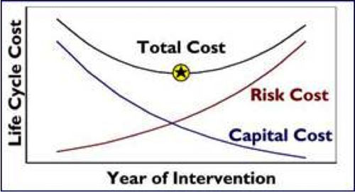
1. The best time to replace an asset is when the total of capital cost and risk cost is lowest. Courtesy BIS Consulting.
This calculation is done bottom-up, making use of input data that the utility’s asset managers have at hand, supplemented by technical expertise: asset health and age, consequences of failure in terms of customer effects, expected maintenance cost, and replacement cost. The process is to get subject-matter experts to make reasonable assumptions about each of these, which then become inputs to an analytical model. Importantly, this means we are asking the experts questions that they understand well: What is the rate of failure for this asset type? What happens to the customers and system if this asset fails? What will it cost to replace the asset?
These are narrow, focused questions within the domain of knowledge of the expert, as opposed to complex economic questions such as, How much underground cable should we replace each year? or, When is the best time to replace this power transformer? Therefore, we are maximizing the value of the subject-matter experts by focusing them on what they understand best, and making explicit, quantitative use of that information.
Customer outage costs are used to assess the dollar consequence cost of failure.
Probability of failure is usually a function of age and condition, often the Health Index. Once we know these, we can quantify risk in dollar terms, and we can identify the point at which the risk of failure is high enough to justify a capital expenditure to replace or refurbish.
Customer outage costs are the most challenging input. The idea is to put ourselves as decision-makers in the shoes of the customer and ask what is their implicit cost when they lose service. It would be nice if we could simply ask them directly, but as John Egan pointed out in his article, it is probably not possible for them to answer effectively.
Ask yourself, if a representative from your utility knocked on your door and asked you how much you’d pay to avoid a two-hour outage, could you give him a meaningful answer? I know I could not. Yet every utility must spend money on its ratepayers’ behalf to avoid outages; no answer is not an option: you either will or will not replace, say, a given power transformer, and that decision implies a certain belief about the cost of an outage. Better to be explicit about your assumptions, so they can be challenged and improved over time and to ensure that there is consistency across all spending decisions.
In my experience, each utility is stuck doing the best it can to decide on a value for customer outage costs. In some cases, these estimates are taken from value models (e.g., UMS Group’s Optimizer, or Davies Group’s Asset Investment System), some make use of customer surveys, and some estimate the value based on judgment. None of these is perfect, but each is transparent and can be used consistently from the bottom of the budgeting process, i.e., estimating remaining life at the asset level, to top-level prioritization.
It is tempting to quantify risk in relative terms, such as “high, medium, low,” or 1 to 10. There are three problems with this. First, this is not very useful in prioritizing expenditures across asset classes. Second, it does not actually identify those assets for which intervention is justified: how many dollars is it worth to move from “high” risk to “medium?” Third, relative measures are opaque to regulators and other parties who need to understand the basis for proposed spending.
Outcomes
The most basic outcome of the economic life process is a long-range projection of the optimal level of spending for each asset class, based on an asset-by-asset assessment of remaining economic life. The histogram in figure 2 shows an example of year-by-year replacement spending for several asset groups. The spike in the first year includes assets who are right at or past their optimal replacement timing. This spike is smoothed over several years. Subsequent years include assets as they reach end of economic life.
Other outcomes include a basis for prioritization explicitly using the trade-off between risk and capital cost; projections of maintenance spending and equipment failures; and snapshots of equipment health, age, criticality, and risk, which are useful for trending.
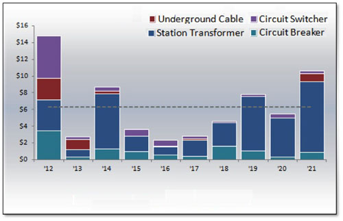
2. Different asset classes require different levels of spending across their lifecycle. Courtesy BIS Consulting.
Other Implications
The total level of spending may be higher or lower than in the past, depending on what the utility’s approach has been. However, the approach described here usually changes the focus of spending toward more critical and higher-risk assets, even though they may not be the oldest or in worst condition. Ironically, the best replacement programs are often not at the most important substations serving the most important loads. These parts of the system usually have high levels of redundancy, meaning the consequences of failure are low. On the other hand, radial systems serving non-critical loads can have very high consequences and are often attractive replacement opportunities.
You can’t say, Oil circuit breakers have a life of 50 years. What you can say is, This oil breaker, installed at this point in our system and facing this risk of failure, has a life of 50 years. But that one over there, in a non-critical location, it has a different life. In other words, service life is asset specific.
There is rarely a “bow wave” of looming replacements. There is often a year-one spike, representing assets that should have been replaced but have not been. This should be less alarming than a “bow-wave” because it suggests the utility is already living in an environment of excess risk, so they know what they’re dealing with. Prioritizing spending to level this spike is important, and the economic life approach allows you to calculate which replacements are most urgent so you can do them first.
- Many utilities have aggressive replacement programs for entire classes of assets, such as direct-buried cable or aging wood poles. Our experience is that programs of this kind often have steep diminishing returns: The first replacements are highly cost effective, but the last ones may actually have negative value because the assets were not yet at end of life. The economic life process is useful first to justify the program by showing the high value of the first replacements, then in managing the scope by showing at what point you should stop it.
- The economic life approach can be used to evaluate the benefit of spares. A spare reduces the consequence of failure, and thus risk, for multiple assets, extending their economic lives. This benefit can be quantified to show whether spares are needed and if so how many.
- Comparison of policy options. For example, many utilities have policies of replacing direct-buried cable with cable in conduit or even concrete-encased conduit. A model of this kind allows you to compare the life-cycle costs of multiple policies to determine which is optimal. It is not always the case that the best option from a technical perspective is the best from the customers’ perspective.
- Grouping assets. Let’s say that the power transformer at a transmission station is at end of life, but the breakers have ten years to go. Is it better to do all the work as part of a single project? If so, when? Now? In ten years? Something in between? This approach allows for comparison of these alternatives to determine which is most cost effective. The basic question is whether the extra cost from replacing some assets at a time other than their optimal is offset by the advantages of a single project.
The economic life approach has been used by unregulated, public utilities (e.g., municipals) to show themselves and their political overseers that the spending they propose provides net value to the stakeholders. It has also been used successfully as part of rate-cases before regulators. In those cases, there is often a lot of back-and-forth, testing of assumptions, etc.
Having an economic life model allows the utility to answer a wide range of questions in a transparent way, producing a high level of confidence in the outcome with the regulator and third-party interveners. The approach has been used by unregulated generation utilities for their own, internal decision-making. They are not responsible to a regulator to justify their spending, but they are responsible to their shareholders.
Does an economic life methodology answer the question raised by John Egan: How can we show our ratepayers that we are providing value to them? Perhaps. But it certainly helps answer the question that must precede that one: How can we show ourselves that we are providing value?
—Darin Johnson is president of BIS Consulting LLC, a firm that offers decision support and risk assessment services.